Optimization:找到最佳解的方式。
若 f'(x) = 0,代表其 x 解點位為 f(x) 極值 (二次函數為 max or min)。
def k(x):
    return -10*(x**2) + (100*x)  + 3

def kd(x):
    return -20*x + 100

from matplotlib import pyplot as plt
x = list(range(0, 11))
y = [k(i) for i in x]
yd = [kd(i) for i in x]     # y 微分後的線段

# 作圖
plt.xlabel('x (time in seconds)')
plt.ylabel('k(x) (height in feet)')
plt.xticks(range(0,15, 1))
plt.yticks(range(-200, 500, 20))
plt.grid()

plt.plot(x, y, 'g', x, yd, 'purple')    # 原有曲線/微分後線
plt.show()
其中要注意的地方是,當 yd=0,即為原曲線的"極值"。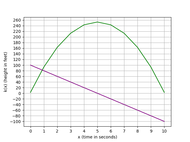
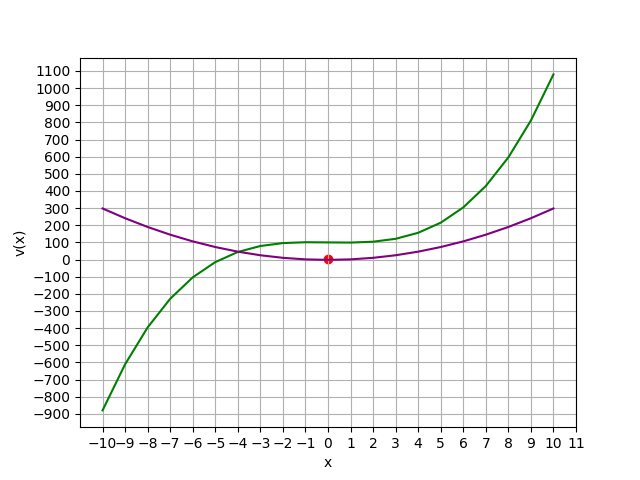
有時 f'(x) = 0 時,並不一定會有 max or min。
def v(x):
    return (x**3) - (2*x) + 100
def vd(x):
    return 3*(x**2) - 2

from matplotlib import pyplot as plt
x = list(range(-10, 11))
y = [v(i) for i in x]
yd = [vd(i) for i in x]

# 作圖
plt.xlabel('x')
plt.ylabel('v(x)')
plt.xticks(range(-10,15, 1))
plt.yticks(range(-1000, 2000, 100))
plt.grid()
plt.plot(x, y, 'g', x, yd, 'purple')
plt.scatter(0, (2/3)**0.5, c='r') # 極值點

plt.show()
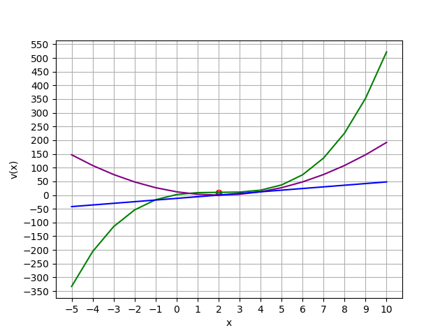
二階導數用於判斷一階導數是 max, min or inflexion
a. 若 f''(x) > 0,表示 f'(x)=0 過後會上升,此函數有最小值。
b. 若 f''(x) < 0,表示 f'(x)=0 過後會下降,此函數有最大值。
c. 若 f''(x) = 0,表示此函數僅有轉折點。
def v(x):
    return (x**3) - (6*(x**2)) + (12*x) + 2
def vd(x):
    return (3*(x**2)) - (12*x) + 12
def v2d(x):
    return (3*(2*x)) - 12

from matplotlib import pyplot as plt
x = list(range(-5, 11))
y = [v(i) for i in x]
yd = [vd(i) for i in x]
y2d = [v2d(i) for i in x]

# 作圖
plt.xlabel('x')
plt.ylabel('v(x)')
plt.xticks(range(-10,15, 1))
plt.yticks(range(-2000, 2000, 50))
plt.grid()

plt.plot(x, y, 'g', x, yd, 'purple', x, y2d, 'b')
plt.scatter(2, v(2), c='r')

plt.show()
自變數 > 1,就叫做梯度非斜率
f(x, y) = x^2 + y^2
f(x, y)/dx = 2x
f(x, y)/dy = 2y
梯度逼近示意圖: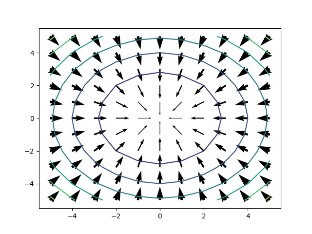
import numpy as np
import matplotlib.pyplot as plt

# 目標函數(損失函數):f(x)
def func(x): return x ** 2 # np.square(x)
# 目標函數的一階導數:f'(x)
def dfunc(x): return 2 * x

def GD(x_start, df, epochs, lr):
    """ 梯度下降法。給定起始點與目標函數的一階導函數,求在epochs次反覆運算中x的更新值
        其原理為讓起始 x = x - dfunc(x)*lr,直到 dfunc(x) = 0,x 就不會再變,求得極值。
        :param x_start: x的起始點
        :param df: 目標函數的一階導函數
        :param epochs: 反覆運算週期
        :param lr: 學習率
        :return: x在每次反覆運算後的位置(包括起始點),長度為epochs+1
     """
    # 此迴圈用作記錄所有起始點用
    xs = np.zeros(epochs+1)     # array[0, 0, ...0] 有1001個
    x = x_start                 # 起始點
    xs[0] = x
    for i in range(epochs):     # i = 0~999
        x += -df(x) * lr        # x = x - dfunc(x) * learning_rate
        xs[i+1] = x
    return xs
# 超參數(Hyperparameters):在模型優化(訓練)前,可調整的參數。
x_start = 2                 # 起始點 (可由任意點開始)
epochs = 1000               # 執行週期數 (程式走多少迴圈停止)
learning_rate = 0.01        # 學習率 (每次前進的步伐多大)

# 梯度下降法
x = GD(x_start, dfunc, epochs, learning_rate)
print(x)
>> [-5. -4. -3.2 -2.56 -2.05 -1.64 -1.31 -1.05 -0.84 -0.67 -0.54 -0.43 -0.34 -0.27 -0.22 -0.18]

from numpy import arange
t = arange(-3, 3, 0.01)
plt.plot(t, func(t), c='b')     # 畫出所求原函數
plt.plot(x, func(x), c='r', label='lr={}'.format(learning_rate)) # 畫出紅連線
plt.scatter(x, func(x), c='r')  # 畫出紅點
plt.legend()

plt.show()
會發現其慢慢逼近 min。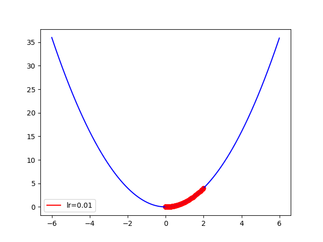
x_start = 5
epochs = 15
learning_rate = 0.01
會發現 Learning rate 太小,根本還沒求到 min 就停止前進。
(可以透過增加 epochs 來達到同樣效果)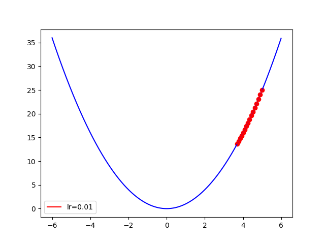
x_start = 5
epochs = 15
learning_rate = 0.9
會發現 Learning rate 太大,逼近速度較快但有跳過最佳解的風險。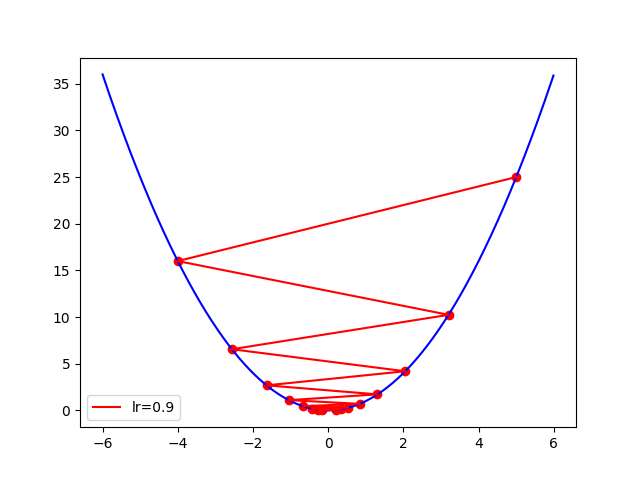
.
積分概念為「函數區域面積總和」。
import matplotlib.pyplot as plt
import numpy as np

# Define function f
def f(x):
    return x
x = range(0, 11)
y = [f(a) for a in x]

# 作圖
plt.xlabel('x')
plt.ylabel('f(x)')
plt.grid()
plt.plot(x, y, color='purple')
p = np.arange(0, 2, 1/20)
plt.fill_between(p, f(p), color='orange')

plt.show()
下圖橘色區塊,即是"函數 f(x)=x 在 x=0~2 間面積。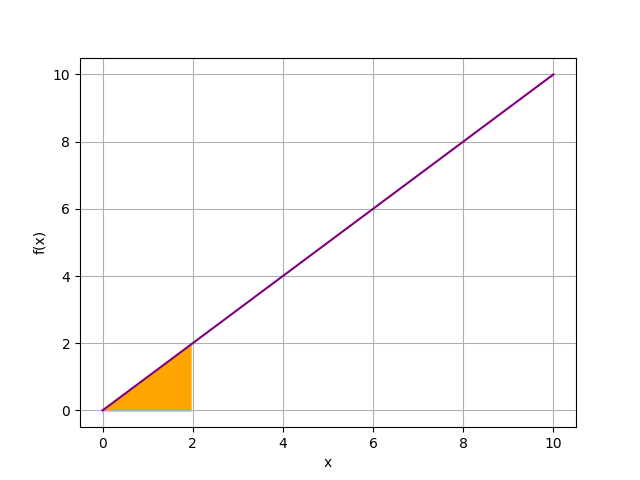
import scipy.integrate as integrate
# Define function f
def f(x):
    return x + 1

# 計算 x=a→b 定積分 intergrate.quad(func, a, b)
i, e = integrate.quad(lambda x: f(x), 0, 2)
i, e    # i 為定積分結果,e 為計算誤差值

>>  4.0 ,  4.440892098500626e-14
利用 numpy 的 inf 計算無窮大,如下:
import scipy.integrate as inte
import numpy as np

i, e = inte.quad(lambda x: np.e**(-5*x), 0, np.inf)
print(i)

>>  0.20000000000000007
nor = lambda x: np.exp(-x**2 / 2.0)/np.sqrt(2.0 * np.pi)
i, e = inte.quad(nor, -np.inf, np.inf)
print('Total Probability:', i)

>>  Total Probability: 0.9999999999999998
i, e = inte.quad(nor, -1, 1)
print('1-sigma:', i)

>>  1-sigma: 0.682689492137086
i, e = inte.quad(nor, -1.96, 1.96)
print('1.96-sigma:', i)

>>  2-sigma: 0.9500042097035591
i, e = inte.quad(nor, -3, 3)
print('3-sigma:', i)
>> 3-sigma: 0.9973002039367399

# 作圖
x = np.linspace(-4, 4, 1000)
y = nor(x)
plt.xlabel('x')
plt.ylabel('Normal Distribution')
plt.grid()

plt.plot(x, y, color='purple')
sig1 = np.linspace(-1, 1, 500)   # 68.3%
sig2 = np.linspace(-2, 2, 500)   # 95.4% (假設檢定常用 2 或 1.96-sigma)
sig3 = np.linspace(-3, 3, 500)   # 99.7%
plt.fill_between(sig3, nor(sig3), color='0.5')
plt.fill_between(sig2, nor(sig2), color='c')
plt.fill_between(sig1, nor(sig1), color='orange')

plt.show()
下圖橘色為 1-sigma,青色為 2-sigma,灰色為 3-sigma。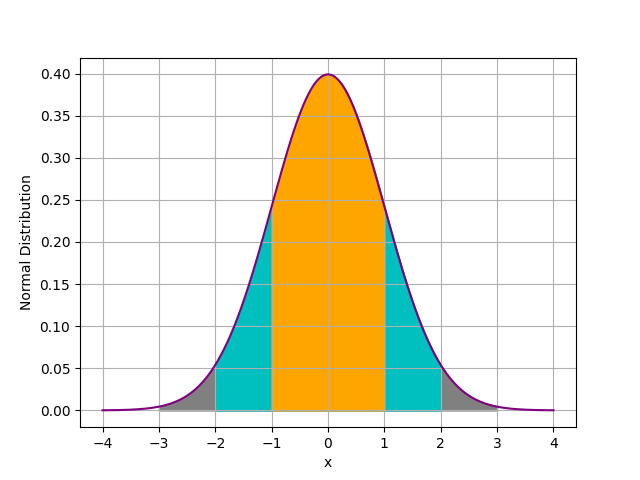
.
.
.
.
.
Ex.1 (2i)(https://reurl.cc/DgbDqe):
(x+2)(x-3) = (x-5)(x-6)
# 2i.
import sympy as sp
x = sp.Symbol('x')
sp.solvers.solve((x+2)*(x-3)-(x-5)*(x-6), x)
>> [18/5]

# 或:
improt sympy as sp
exp1='(x+2)*(x-3), (x-5)*(x-6)'
sp.solvers.solve(sp.core.sympify(f"Eq({exp1})"))
>> [18/5]
Ex.2 (3c)(https://reurl.cc/DgbDqe):
|10-2x| = 6
# 若要計算絕對值,須加上 real=True
x = sp.Symbol('x', real=True) # real=True 表 x 是實數
sp.solvers.solve(abs(10-2*x)-6, x))
>> [2 8]
Ex.3 (3c)(https://reurl.cc/EnbDQk):
4x + 3y = 4
2x + 2y - 2z = 0
5x + 3y + z = -2
# 1. numpy 解法
import numpy as np
left = str(input("請輸入等號左測導數 (以','逗號隔開): "))
left = left.split(',')
left = list(map(int, left))

right = str(input("請輸入等號右測導數 (以','逗號隔開): "))
right = right.split(',')
right = list(map(int, right))

a_shape = int(len(left)**0.5)  # 得到矩陣形狀
a = np.array(left).reshape(a_shape, a_shape) # 重整矩陣為正方形
b = np.array(right)
np.linalg.solve(a, b)
>> 請輸入等號左測導數 (以','逗號隔開): 4,3,0,2,2,-2,5,3,1
>> 請輸入等號右測導數 (以','逗號隔開): 4,0,-2
>> [-11.  16.   5.]

# 2. sympy 解法
from sympy.solvers import solve
eq = []
while True:
    inp = input('請輸入方程式: ')
    if inp =='':
        break
    eq.append(inp)
if len(eq)>0:
    for i in range(len(eq)):
        arr = eq[i].split('=')
        if len(arr) ==2:
            eq[i] = arr[0] + '-(' + arr[1] + ')'
    solve(eq)
>> 請輸入方程式: 4x + 3y = 4
>> 請輸入方程式: 2x + 2y - 2z = 0
>> 請輸入方程式: 5x + 3y + z = -2
>> 請輸入方程式:
>> {x: -11, y: 16, z: 5}
from sympy.solvers import solve

def run():
    eq_clean = []
    exp = text.get('1.0', 'end')    # 把輸入區塊的東西丟進 exp
    eq = exp.split('\n')            # 用 '\n' 拆分
    if len(eq) > 0:                 # 若輸入的東西不是空白的
        for i in range(len(eq)):    # i = 輸入幾個多項式
            if eq[i] == '':
                continue
            arr = eq[i].split('=')  # arr = 每個多項式用 '=' 拆分
            if len(arr) == 2:       # 若只有兩項 (也就是只有等號左右側)
                eq[i] = arr[0] + '-(' + arr[1] + ')'
            eq_clean.append(eq[i])  # 把 eq[0] 加入 eq_clean
        ans.set(solve(eq_clean))    # 把 eq_clean 丟進 sympy 求解,放入變數 ans
接著我們設計彈出視窗 (tkinter):
import tkinter as tk

# 1. 宣告一個根視窗
root = tk.Tk()

# 2. 建立顯示字元區塊
# text= : 顯示字元
# height=1 : 高度為1
# font= : 字體 大小 粗體
tk.Label(root, text='請輸入方程式: (2x 須輸入 2*x)', height=1, font='Helvetic 18 bold').pack(fill=tk.X)

# 3. 建立可輸入區塊
text = tk.Text(root, height=5, width=30, font='Helvetic 18 bold')
text.pack()

# 4. 建立按紐觸發 run() 函數
# commend= : 事件處理,通常會接一個函數
tk.Button(root, text='求解', font='Helvetic 36 bold', command=run).pack(fill=tk.X)

# 5. 建立顯示答案區塊
# textvariable= : 需求顯示的字元
ans = tk.StringVar()
tk.Label(root, text='', height=1, font='Helvetic 18 bold', textvariable=ans).pack(fill=tk.X)

# 6. 監聽事件
root.mainloop()
實際畫面如下: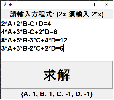
當然,可以用網頁設計輸入畫面,會更簡潔:
import streamlit as st
# 要用 cmd : streamlit run f:/LessonOnClass/Part2/20210417/00.Practice.py
import sympy as sp

x, y, z = sp.symbols('x y z')

exp = st.text_area('請輸入聯立方程式: ', 'x+y=5\nx-y=1') # title1
st.markdown('# 聯立方程式求解') # title2

if st.button('求解'):   # 若按下按鈕則執行以下
    eq_c = []
    eq = exp.split('\n')
    if len(eq)>0:
        for i in range (len(eq)):
            if eq[i] == '':
                continue
            arr = eq[i].split('=')
            if len(arr) ==2:
                eq[i] = arr[0] + '-(' + arr[1] + ')'
            eq_c.append(eq[i])
    ans = sp.solvers.solve(eq_c)
    st.write(f'結果: {ans}')   # 將 ans 寫入網頁中
實際畫面如下:
利用梯度下降法,求得目標函數 f(x) 的區域內極值。
f(x) = x^3 - 2x + 100
f(x) = -5x^2 + 3x + 6
f(x) = 2x^4 - 3x^2 + 2x - 20
f(x) = sin(x)E*(-0.1*(x-0.6)**2)
*提示:用 y_prime = y.diff(x) 求微分後方程式。
 s790502ss

 iThome鐵人賽