在每個 Fold 中，讓模型用 predict_proba 輸出機率，並將機率值 (針對 Target=1 的機率) 存入 y_pred 中，方便後續回測使用。

def walk_forward_train(X, y, df, train_window=2000, test_window=400, step=400, model_cls=RandomForestClassifier, model_kwargs=None):
    """
    sliding-window walk-forward training.
    - train_window: 用多少筆資料訓練
    - test_window: 每次測試用多少筆
    - step: 每次往前移動多少筆 (通常 = test_window)
    """
    if model_kwargs is None:
        model_kwargs = {"n_estimators":200, "random_state":42,  "class_weight": "balanced"}

    n = len(X)
    folds = []
    f1_scores = []
    last_model = None
    last_test_index = None
    last_y_true = None
    last_y_proba = None
    last_y_hard_pred = None     #儲存硬預測 (0或1)，用於分類報告

    start = 0
    # 從 train_window 開始，確保有足夠訓練資料
    while start + train_window + test_window <= n:
        train_idx = list(range(start, start + train_window))
        test_idx = list(range(start + train_window, start + train_window + test_window))

        X_train, X_test = X.iloc[train_idx], X.iloc[test_idx]
        y_train, y_test = y.iloc[train_idx], y.iloc[test_idx]

        model = model_cls(**model_kwargs)
        model.fit(X_train, y_train)

        # 計算硬預測 (y_hard_pred) 和機率 (y_proba)
        y_hard_pred = model.predict(X_test)         # 0 或 1
        y_proba = model.predict_proba(X_test)[:, 1] # 0.0 到 1.0

        #計算 Target=1 (pos_label=1) 的 F1-Score
        f1 = f1_score(y_test, y_hard_pred, pos_label=1, zero_division=0)
        f1_scores.append(f1)

        # move window
        start += step

        # 儲存最後一個 Fold 的結果
        last_model = model
        last_test_index = test_idx
        last_y_true = y_test
        last_y_proba = y_proba          # 👈 傳出機率 (P_proba)
        last_y_hard_pred = y_hard_pred # 👈 傳出硬預測 (P_hard)

        folds.append({
            "train_index": train_idx,
            "test_index": test_idx,
            "model": model,
            "y_true": y_test,
            "y_proba": y_proba,    # 儲存機率
            "y_pred": y_hard_pred, # 儲存硬預測 (舊的 y_pred)
            "f1_score": f1
        })

    print(f"\nWalk-forward 訓練完成。共 {len(f1_scores)} 個 Fold。")

    if f1_scores:
        avg_acc = np.mean(f1_scores)
        print(f"📊 平均準確率: {avg_acc:.4f}")
    else:
        # 如果 scores 為空，則平均準確率為 N/A
        print("📊 平均準確率: N/A (無 Fold 執行)")

    if not folds:
        print("❌ 錯誤：Walk-forward 沒有執行任何 Fold。請檢查資料量是否足夠。")
        return None, None, None, None, None
    
    #新增分類報告，以量化模型在類別不平衡下的性能
    from sklearn.metrics import classification_report
    
    if last_y_hard_pred is not None and len(last_y_hard_pred) > 0:
        acc_last_fold = accuracy_score(last_y_true, last_y_hard_pred)
        print(f"✅ 最後一個 Fold 總準確率: {acc_last_fold:.4f}")
        print("\n=== 最後一個 Walk-forward 區段的詳細分類報告 (Target=1: 預測漲幅>0.15%) ===")
        print(classification_report(last_y_true, last_y_hard_pred, 
                                     target_names=['Target=0 (Down/Small)', 'Target=1 (Up)'], 
                                     zero_division=0))
    
    # 使用最後一個 Fold 的結果繪製預測圖
    plot_predictions(df, last_y_true, last_y_hard_pred, last_test_index, f"Predictions vs Actual (Latest {test_window} bars)")

    return last_model, last_test_index, last_y_true, last_y_proba, last_y_hard_pred, folds

walk_forward_train 傳遞回來的 y_pred 已經是機率值。需要在回測中引入一個 信心閾值 (CONFIDENCE_THRESHOLD)。

def backtest_strategy(df, y_true, y_proba, test_index,
                         initial_capital=10000,
                         position_size_ratio=0.1,
                         fee_rate=0.001,
                         atr_multiplier=1.5,
                         take_profit_ratio=0.02,
                         debug=False,
                         confidence_threshold=0.60):    #新增信心閾值
    """
    改進版策略回測：
    - 支援多空進出場
    - 含 ATR 止損與獲利邏輯
    - 加入最終平倉
    - 修正 equity 曲線與手續費
    """
    df_test = df.iloc[test_index].copy().reset_index(drop=True)
    df_test["True"] = pd.Series(y_true).reset_index(drop=True)
    df_test["Proba"] = pd.Series(y_proba).reset_index(drop=True)

    balance = initial_capital
    equity_curve = [balance]
    trades = []
    position, entry_price, entry_capital, entry_units = None, 0, 0, 0

    for i in range(1, len(df_test)):
        price_now = df_test["close"].iloc[i]
        rsi = np.nan_to_num(df_test["RSI"].iloc[i], nan=50)

        proba = df_test["Proba"].iloc[i - 1]

        atr = np.nan_to_num(df_test["ATR"].iloc[i], nan=0)

        # -------------------
        # 1️⃣ 進場邏輯
        # -------------------
        if position is None:
            if proba >= confidence_threshold and rsi > 55:
                position = "long"
                entry_price = price_now
                entry_capital = balance * position_size_ratio
                entry_units = entry_capital / entry_price
                balance -= entry_capital * fee_rate  # 手續費
                if debug:
                    print(f"[BUY] @ {price_now:.2f}, Proba={proba:.2f}")

            elif (1 - proba) >= confidence_threshold and rsi < 45:
                position = "short"
                entry_price = price_now
                entry_capital = balance * position_size_ratio
                entry_units = entry_capital / entry_price
                balance -= entry_capital * fee_rate
                if debug:
                    print(f"[SELL] @ {price_now:.2f}, Proba={proba:.2f}")

        # -------------------
        # 2️⃣ 出場邏輯
        # -------------------
        elif position == "long":
            change = (price_now - entry_price) / entry_price
            stop_loss = -atr_multiplier * atr / entry_price
            take_profit = take_profit_ratio
            if change <= stop_loss or change >= take_profit:
                pnl = entry_capital * change
                balance += entry_capital + pnl - (entry_capital + pnl) * fee_rate
                trades.append(pnl / entry_capital)
                if debug:
                    print(f"[EXIT LONG] @ {price_now:.2f}, PnL={pnl/entry_capital:.2%}")
                position, entry_capital, entry_units = None, 0, 0

        elif position == "short":
            change = (entry_price - price_now) / entry_price
            stop_loss = -atr_multiplier * atr / entry_price
            take_profit = take_profit_ratio
            if change <= stop_loss or change >= take_profit:
                pnl = entry_capital * change
                balance += entry_capital + pnl - (entry_capital + pnl) * fee_rate
                trades.append(pnl / entry_capital)
                if debug:
                    print(f"[EXIT SHORT] @ {price_now:.2f}, PnL={pnl/entry_capital:.2%}")
                position, entry_capital, entry_units = None, 0, 0

        # -------------------
        # 3️⃣ 記錄淨值 (Equity)
        # -------------------
        current_equity = balance
        if position == "long":
            current_equity += entry_capital * ((price_now - entry_price) / entry_price)
        elif position == "short":
            current_equity += entry_capital * ((entry_price - price_now) / entry_price)

        equity_curve.append(current_equity)

    # -------------------
    # 4️⃣ 最後平倉 (Final Closeout)
    # -------------------
    if position is not None:
        final_price = df_test["close"].iloc[-1]
        if position == "long":
            pnl = entry_capital * ((final_price - entry_price) / entry_price)
        else:
            pnl = entry_capital * ((entry_price - final_price) / entry_price)
        balance += entry_capital + pnl - (entry_capital + pnl) * fee_rate
        trades.append(pnl / entry_capital)
        if debug:
            print(f"[FORCED EXIT] {position.upper()} @ {final_price:.2f}, Final PnL={pnl/entry_capital:.2%}")

    # -------------------
    # 5️⃣ 結果與報表
    # -------------------
    if len(equity_curve) < len(df_test):
        equity_curve += [balance] * (len(df_test) - len(equity_curve))
    df_test["Equity"] = equity_curve

    total_return = (balance / initial_capital - 1) * 100
    max_drawdown = ((df_test["Equity"].cummax() - df_test["Equity"]) / df_test["Equity"].cummax()).max() * 100
    win_rate = (sum([1 for t in trades if t > 0]) / len(trades)) * 100 if trades else 0

    # -------------------
    # 6️⃣ 繪製曲線
    # -------------------
    plt.figure(figsize=(12, 6))
    plt.plot(df_test["timestamp"], df_test["Equity"], label="Equity Curve", color="blue")
    plt.axhline(initial_capital, linestyle="--", color="gray", alpha=0.7)
    plt.title("Backtest Equity Curve (v2 Improved)")
    plt.xlabel("Time") # 保持 Time 標籤
    plt.ylabel("Capital (USDT)")
    plt.legend()
    plt.xticks(rotation=45) # 加上旋轉，避免時間標籤重疊
    plt.tight_layout()
    plt.show()

    # -------------------
    # 7️⃣ 印出統計
    # -------------------
    print(f"💰 最終資金: {balance:.2f} USDT")
    print(f"📈 總報酬率: {total_return:.2f}%")
    print(f"📉 最大回撤: {max_drawdown:.2f}%")
    print(f"✅ 勝率: {win_rate:.2f}%")
    print(f"📊 交易次數: {len(trades)}")

    return df_test, trades

修改主程式

if __name__ == "__main__":
    # 變數初始化
    model, last_test_index, y_true, last_y_proba, last_y_hard_pred, folds = None, None, None, None, None, None

    # 設定資料時間範圍
    START_DATE = "2025-06-01"   # 想從哪一天開始抓
    TIMEFRAME = "1h"

    # 根據起始日期自動計算 TOTAL_LIMIT
    TOTAL_LIMIT = calc_total_limit(START_DATE, timeframe=TIMEFRAME)

    # Walk-forward 預設參數 (固定這兩個，讓 TRAIN_WINDOW 變化)
    TARGET_FOLDS = 7
    FIXED_TEST_WINDOW = 300
    FIXED_STEP = 300
    RETURN_THRESHOLD = 0.0015 # 0.15% 漲幅才算 Target=1

    # 新增信心閾值
    CONFIDENCE_THRESHOLD = 0.60 # 60% 信心才進場 (這是一個優化參數)

    print(f"===== 抓取與處理資料 (總筆數: {TOTAL_LIMIT}) =====")

    # 加入 force_reload=True 以確保抓取足夠數據】
    df_raw = fetch_crypto_data(
        symbol="BTC/USDT",
        timeframe="1h",
        start_date=START_DATE,   # 從這天開始抓資料
        force_reload=True
    )

    #加入技術指標與 ML 資料處理
    df_ind = add_indicators(df_raw)
    X, y, df = prepare_ml_data(df_ind, return_threshold=RETURN_THRESHOLD)

    #計算 Walk-forward 參數
    FINAL_DATA_LEN = len(X)

    TRAIN_WINDOW, TEST_WINDOW, STEP, ACTUAL_FOLDS = calculate_walk_forward_params(
        total_data_len=FINAL_DATA_LEN,
        target_folds=TARGET_FOLDS,
        fixed_test_window=FIXED_TEST_WINDOW,
        fixed_step=FIXED_STEP
    )
    
    if ACTUAL_FOLDS < 1:
        print("\n❌ 錯誤：數據量嚴重不足，無法執行 Walk-forward 訓練。請將 START_DATE 設置得更早。")

    else: 
        print("\n===== 開始 Sliding-Window Walk-forward 訓練 =====")
        # 傳遞 TRAIN_WINDOW, TEST_WINDOW, STEP 參數
        model, last_test_index, y_true, last_y_proba, last_y_hard_pred, folds = walk_forward_train(
            X, y, df,
            train_window=TRAIN_WINDOW, 
            test_window=TEST_WINDOW, 
            step=STEP
        )

    # 確保只有在有結果時才嘗試回測 (解決您之前的 TypeError)
    if model is not None:
        print("\n===== 回測最後一個 Walk-forward 區段的績效 =====")
        df_test, trades = backtest_strategy(
            df, 
            y_true.astype(int), 
            last_y_proba, 
            last_test_index,
            confidence_threshold = CONFIDENCE_THRESHOLD
        )
        
        print(f"\n✅ 系統已使用 {len(folds)} 個 Fold 訓練並完成回測。")
    else:
        print("\n⚠️ 因數據量不足，無法執行回測。")

以下是執行後的結果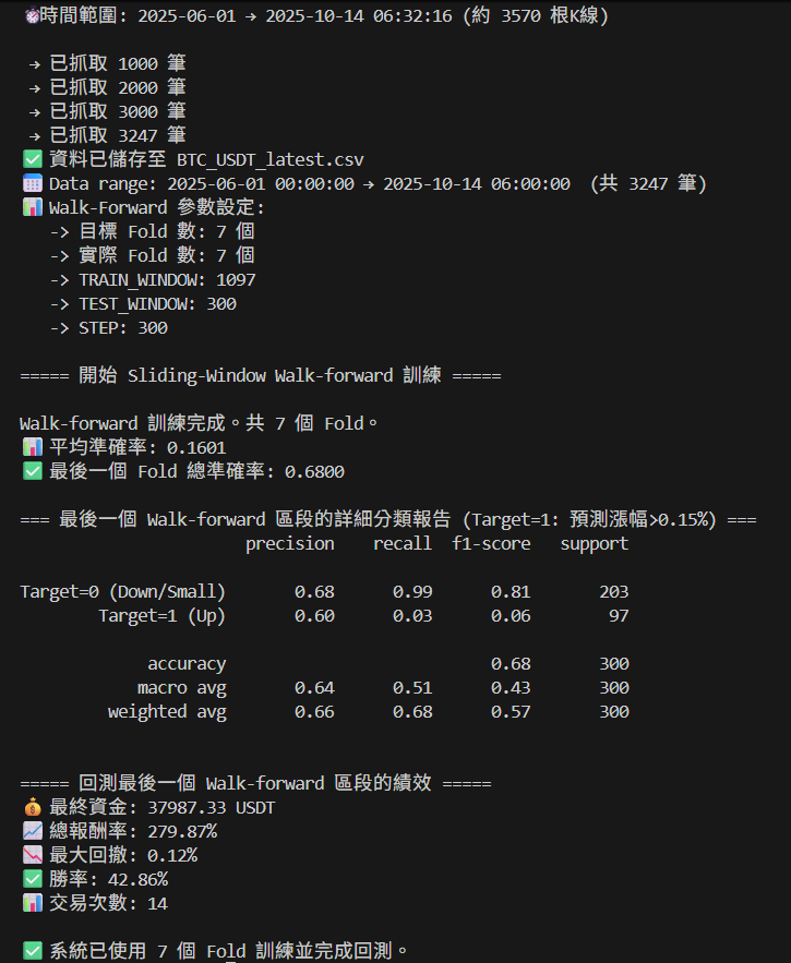

Precision (精確度) 從一開始的0.24到上次優化後的0.29再到這次優化後的0.60可以說大幅提升。
Recall (召回率) 從一開始的0.14到上次優化後的0.32再到這次優化後的0.03幾乎崩潰了，不敢猜漲。
F1_Score也跌到谷底。
所以下一步我要拯救我的Recall，移除極端平衡，導入機率濾網。