Python 演算法 Day 13 - Ensemble Learning

自學筆記

s790502ss 2021-12-21 15:24:15 ‧ 3504 瀏覽

分享至

Chap.II Machine Learning 機器學習

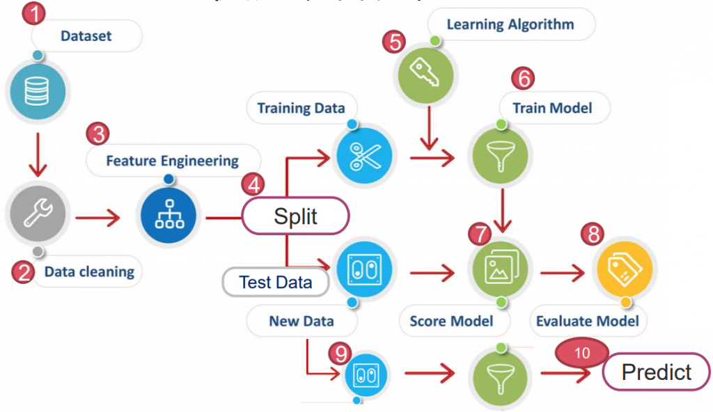
https://yourfreetemplates.com/free-machine-learning-diagram/

Part 3. Learning Algorithm 演算法

上一章提到的基礎學習（又稱弱學習）於多數真實情況下的性能其實並不好。
低維資料時具有較高的標準差，高維資料時則是變異太大導致穩定性不夠。
為了降低模型變異及提高準確度，可根據不同的數據，於各階段使用不同的演算法來訓練模型。
最終以不同權重的方式結合每個結果，得到一個更優性能的學習器。

3-2. Ensemble Learning 集成學習

核心理念：透過組合多個弱學習器，從而創建一個強學習器（或稱「集成學習」）。
當數據非常複雜，或有多種潛在的假設時，集成學習非常實用。

A. Majority Voting 多數投票法

這是最簡單的集成學習。
將資料丟進 n 個「不同的弱學習器」，求出測試資料的預測結果，將結果向量相加。
因為分類只有 0/1，新的結果向量裡的值最大為 n，最小為0。
透過投票，至少有過半數以上的學習器預測 1，才判定結果是 1，其餘則為 0。

投票方法又分兩種：
硬投票：預測結果是所有投票結果最多出現的類。
軟投票：預測結果是所有投票結果中「概率和」最大的類。
如：預測某樣本的結果為 70%、51%、1%，硬投票會判定為正樣本（2 正 1 負），但軟投票則會判定為負樣本（70%+51%+1% < 30%+49%+99%）。

優點：簡單快速，不需調整過多參數。
缺點：學習器種類上限會限制其精確度。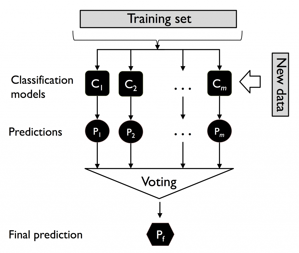

以鳶尾花為例，且故意拿掉部分 y 與特徵（使模型預測較不準）：

from sklearn import datasets
from sklearn.preprocessing import LabelEncoder
from sklearn.model_selection import train_test_split

ds = datasets.load_iris()
X, y = ds.data[50:, [1, 2]], ds.target[50:]
y = LabelEncoder().fit_transform(y)

X_train, X_test, y_train, y_test = train_test_split(X, y, test_size=0.5, random_state=1, stratify=y)

# 三個弱學習器：此處用邏輯斯迴歸、決策樹和 KNN
from sklearn.pipeline import make_pipeline
from sklearn.preprocessing import StandardScaler
from sklearn.linear_model import LogisticRegression
from sklearn.tree import DecisionTreeClassifier
from sklearn.neighbors import KNeighborsClassifier 
from sklearn.model_selection import cross_val_score
from sklearn.ensemble import RandomForestClassifier

lr_PL = make_pipeline(
    StandardScaler(),
    lr = LogisticRegression(penalty='l2',　C=0.001,　random_state=1)
)
dt_PL = make_pipeline(
    DecisionTreeClassifier(max_depth=1,　criterion='entropy',　random_state=0)
)
knn_PL = make_pipeline(
    StandardScaler(),
    KNeighborsClassifier(n_neighbors=1, metric='minkowski')
)

all_clf = [lr_PL, dt_PL, knn_PL]

多數投票法：此處使用軟投票

from sklearn.ensemble import VotingClassifier
ens = [('LR', lr_PL), ('DT', dt_PL), ('KNN', knn_PL)]
vc = VotingClassifier(ens, voting='soft')

clf_labels = ['Logistic regression', 'Decision tree', 'KNN', 'Voting Classifier']
all_clf = [lr_PL, dt_PL, knn_PL, vc]

# 使用 cross validation 避免過擬合
from sklearn.model_selection import cross_val_score
for clf, label in zip([lr_PL, dt, knn_PL], clf_labels):
    scores = cross_val_score(
        clf, X_train, y_train,
        cv=10,
        scoring='roc_auc'
    )
    print(f"ROC AUC: {scores.mean():0.2f} (+/- {scores.std():0.2f}) [{label}]")
    
>>  ROC AUC: 0.92 (+/- 0.15) [Logistic regression]
    ROC AUC: 0.87 (+/- 0.18) [Decision Tree]
    ROC AUC: 0.85 (+/- 0.13) [KNN]
    ROC AUC: 0.98 (+/- 0.05) [Voting Classifier]

把決策邊界作圖（代碼在補充 1.）：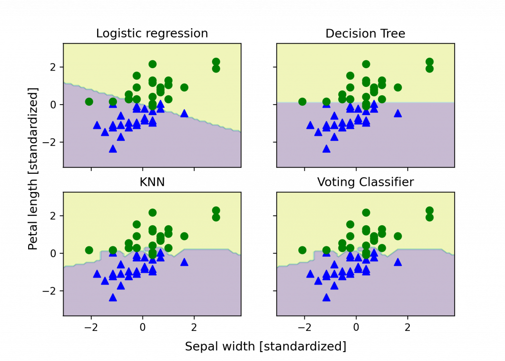

看起來成效卻實比單個學習器還好！

B. Bagging 裝袋法

直接投票法的問題－學習器種類有限，僅憑數個演算法，可能無法達到專案需求的精度。
因此，人們發明 Bootstrap AGGregatING，也就是 Bagging 裝袋法來解決。

選定一弱學習器。將原樣本做「會放回抽樣」，生成 n 個與原數據一樣大的「自助樣本」。
（因此，某些樣本點可能在自助樣本中出現多次，某些則被忽略）
學習器會將每個自助樣本都訓練，最終產出 n 個模型。藉投票決定將測試樣本分派（預測）到哪個類別。

優點：從樣本隨機抽樣，降低雜訊被重複訓練到的機率，進而提升模型穩定性。
缺點：只是將每次的錯誤率稀釋掉，實際模型依舊沒有學的更好。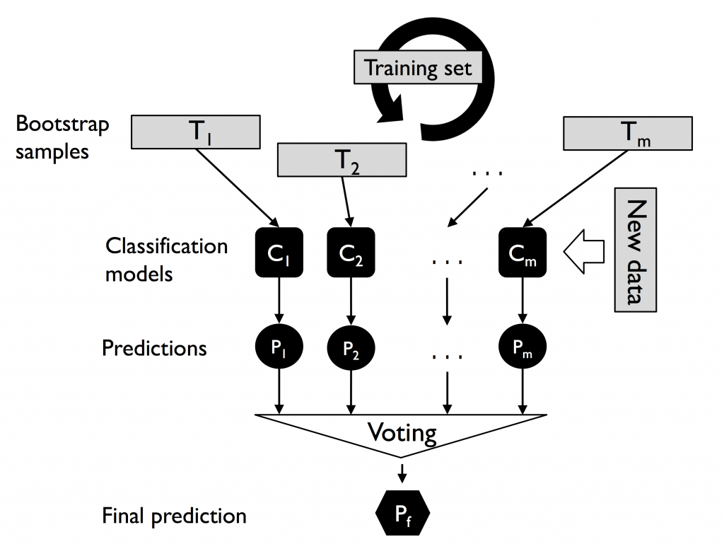

以紅酒分類為例：

from sklearn.datasets import load_wine
X, y = load_wine(return_X_y=True)

from sklearn.preprocessing import LabelEncoder
from sklearn.model_selection import train_test_split
le = LabelEncoder()
y = le.fit_transform(y)

X_train, X_test, y_train, y_test = train_test_split(X, y, test_size=0.2, random_state=1, stratify=y)

B1. Bagging：此處使用決策樹做 Bagging（其實就是隨機森林）

from sklearn.tree import DecisionTreeClassifier
from sklearn.ensemble import BaggingClassifier

tree = DecisionTreeClassifier(criterion='entropy', random_state=1)
bag = BaggingClassifier(
    base_estimator=tree,
    n_estimators=500,
    max_samples=1.0,
    max_features=1.0,
    bootstrap=True,
    bootstrap_features=False,
    n_jobs=1,
    random_state=1
)

超參數：
1. nestimators: 創建 n 個子模型。默認 10。
2. maxsamples: 每個子模型使用 n 個樣本數據訓練。默認 1.0。
3. maxfeatures: 若是 int，則選取 n 個特徵；若是 float 則選取 n\X.shape[1] 個特徵。默認 1.0。
4. bootstrap: 在隨機選取樣本時是否將已選樣本放回。默認 True。
5. bootstrapfeatures: 在隨機選取特徵時是否將已選特徵放回。默認 False。
6. njobs: 用於訓練和預測所需要 CPU 的數量（-1 表使用所有空閒 CPU）。

接著比較一下一般決策樹 vs. Bagging 決策樹（就是隨機森林）

# 1. 決策樹
from sklearn.metrics import accuracy_score

tree.fit(X_train, y_train)
y_train_pred = tree.predict(X_train)
y_test_pred = tree.predict(X_test)

tree_train = accuracy_score(y_train, y_train_pred)
tree_test = accuracy_score(y_test, y_test_pred)
print(f'Decision tree train/test accuracies {tree_train:.3f} / {tree_test:.3f}')

# 2. Bagging
bag.fit(X_train, y_train)
y_train_pred = bag.predict(X_train)
y_test_pred = bag.predict(X_test)

bag_train = accuracy_score(y_train, y_train_pred) 
bag_test = accuracy_score(y_test, y_test_pred) 
print(f'Bagging train/test accuracies {bag_train:.3f} / {bag_test:.3f}')

>>  Decision tree train/test accuracies 1.000 / 0.833
    Bagging train/test accuracies 1.000 / 0.917

把決策邊界作圖（代碼在補充 2.）：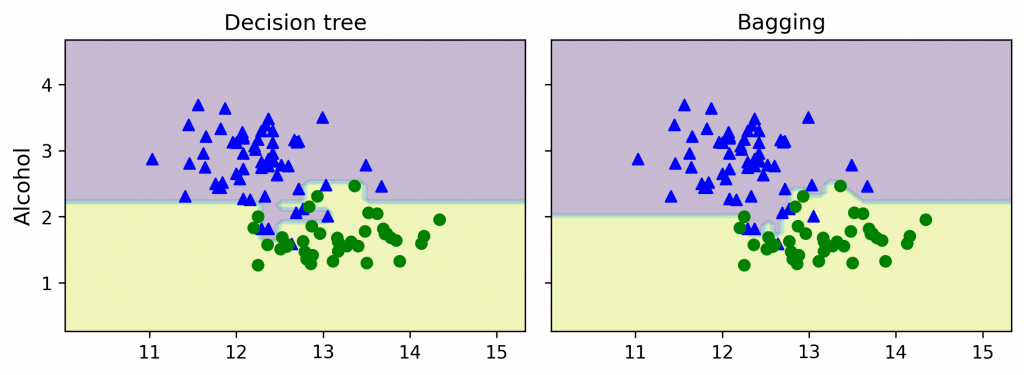

B2. Random Forest 隨機森林法

基於決策樹演算法上，透過 Bagging 演算法，讓多顆樹生長且不進行剪枝，
並對這些樹的結果進行組合（分類用簡單多數投票法，迴歸則用平均法）。

優點：可以處理分類與迴歸資料。接受高維度資料。非平衡誤差資料時能平衡誤差。
缺點：需大量記憶體儲存每顆樹的資訊。無法針對單一顆樹作解釋。

from sklearn.datasets import load_boston
ds = datasets.load_breast_cancer()
X=pd.DataFrame(ds.data, columns=ds.feature_names)
y=pd.DataFrame(ds.target, columns=['Cancer'])

from sklearn.model_selection import train_test_split
X_train, X_test, y_train, y_test = train_test_split(X, y, test_size = 0.3)

from sklearn.ensemble import RandomForestClassifier as RFC
rfc = RFC(n_estimators=100, criterion='gini', max_depth=3, random_state=1)

超參數：
1. nestimators: 要種幾棵樹。默認 100。
2. criterion: 不純度方法，'gini' & 'entropy'。默認 gini。
3. maxdepth: 樹的分裂層數。若 None，則擴展節點至所有葉 minsamplessplit 樣本。默認 None。
4. minsamplessplit: 分裂一個內部節點所需的最小樣本數。默認 2。

rfc.fit(X_train, y_train)
rfc.score(X_test, y_test)

>>  0.9415204678362573

C. Boosting 強化法

Boosting 是指能夠將弱學習器轉化爲強學習器的一系列算法。
概念類似 Bagging，不同的是，它會將前一次學習器「分類錯誤的資料」的權重提高，以訓練下一次。
學習器會學習到上一次「錯誤分類資料」的特性，進而提升分類結果。

優點：一般來說可得到比 Bagging 更好的結果。
缺點：若原生資料集雜訊太多，易使模型放大對雜訊的判斷，導致結果失準。

C1. AdaBoost

以紅酒分類為例，：

from sklearn.datasets import load_wine
X, y = load_wine(return_X_y=True)

from sklearn.preprocessing import LabelEncoder
from sklearn.model_selection import train_test_split
le = LabelEncoder()
y = le.fit_transform(y)

X_train, X_test, y_train, y_test = train_test_split(X, y, test_size=0.2, random_state=1, stratify=y)

Boosting：此處使用決策樹做 Boosting

from sklearn.tree import DecisionTreeClassifier
from sklearn.ensemble import AdaBoostClassifier

tree = DecisionTreeClassifier(criterion='entropy', max_depth=1, random_state=1)
ada = AdaBoostClassifier(
    base_estimator=tree,
    n_estimators=500, 
    learning_rate=0.01,
    random_state=1
)

超參數：
1. nestimators: 創建 n 個學習器。默認 50。
2. learningrate: 學習速率。默認 1.0。

接著比較一下一般決策樹 vs. Boosting 決策樹

from sklearn.metrics import accuracy_score
tree.fit(X_train, y_train)

y_train_pred = tree.predict(X_train)
y_test_pred = tree.predict(X_test)

tree_train = accuracy_score(y_train, y_train_pred)
tree_test = accuracy_score(y_test, y_test_pred)
print(f'Decision tree train/test accuracies {tree_train:.3f}/{tree_test:.3f}')

ada.fit(X_train, y_train)
y_train_pred = ada.predict(X_train)
y_test_pred = ada.predict(X_test)

ada_train = accuracy_score(y_train, y_train_pred) 
ada_test = accuracy_score(y_test, y_test_pred) 
print(f'AdaBoost train/test accuracies {ada_train:.3f}/{ada_test:.3f}')

>>  Decision tree train/test accuracies 0.916/0.875
    AdaBoost train/test accuracies 0.968/0.917

把決策邊界作圖（代碼在補充 3.）：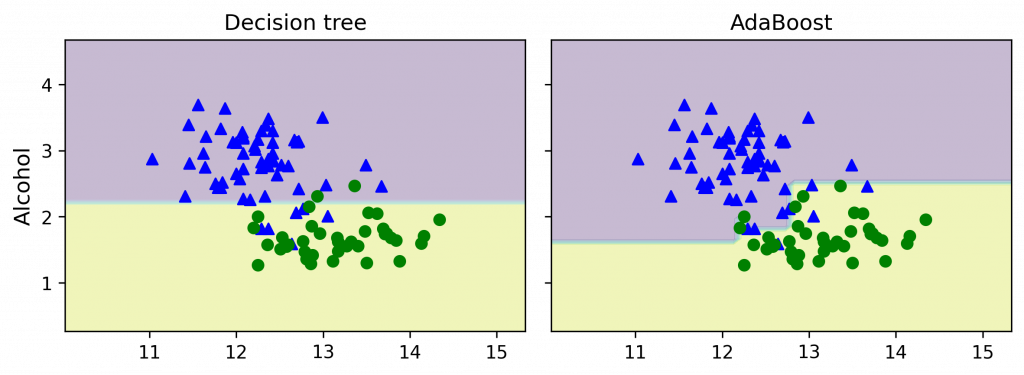

C2. Gradient Boosting 梯度強化法

其原理與 Ada 類似，差別在前者利用「分類錯誤資料」權重定位模型的不足，後者則是透過「梯度」。
原理可參考文章 1、文章 2 & 文章 3

最有名的莫過於是 XGBoost。
XGBoost 全名 eXtreme Gradient Boosting，是 Kaggle 競賽中常見的演算法。
它保有 Gradient Boosting 的做法，使後生成樹能修正前棵樹的錯誤。
此外，如隨機森林，生成每棵樹時會隨機抽取特徵，使每棵樹的生成不會拿全部的特徵參與決策。
故可實現平行處理。並不是說可以平行處理多顆樹，而是指它可平行處理特徵選取的計算。
可說是同時結合 Bagging 和 Boosting 的優點。

為抑制模型複雜化，XGboost 在目標函數添加了 Regularization。
模型在訓練時為了擬合訓練資料，會產生很多高次項的函數，但反而容易被雜訊干擾導致過度擬合。
因此 L1/L2 使損失函數更平滑，抗雜訊干擾能力更大。

最後 XGboost 用到了一 & 二階導數來生成下一棵樹。
其中 Gradient 就是所謂的一階導數，而 Hessian 即為二階導數。

優點：準確率高。支援平行處理。抗過擬合與抗雜訊能力強。

# 同樣用上面的酒類分類
from sklearn.tree import DecisionTreeClassifier
from xgboost import XGBClassifier

tree = DecisionTreeClassifier(criterion='entropy', max_depth=1, random_state=1)
xgb = XGBClassifier(
    n_estimators=500, 
    learning_rate=0.01,
    random_state=1
)

超參數：
1. nestimators: 創建 n 個學習器。
2. maxdepth: 樹的最大深度，（通常設計 3~10）。默認 6。
3. booster: gbtree 樹模型（默認） / gbliner 線性模型。
4. learningrate: 學習速率，（通常設計 0.01~0.2）。默認 0.3。
完整可看: https://www.twblogs.net/a/5db37e49bd9eee310ee694ee

Stacking 黏合法

與前面 Baggin / Boosting 不同，Stacking 會有兩種模型：

Base-Models: 用於訓練數據並預測資料。
Meta-Model : 用於結合 Base-Models 預測的資料，得出最終預測模型。

同樣用上面的酒類分類：

from sklearn.pipeline import make_pipeline
from sklearn.preprocessing import StandardScaler
from sklearn.tree import DecisionTreeClassifier
from sklearn.neighbors import KNeighborsClassifier
from sklearn.linear_model import LogisticRegression
from sklearn.ensemble import StackingClassifier

tree = DecisionTreeClassifier(criterion='entropy', max_depth=1, random_state=1)

knn_PL = make_pipeline(
    StandardScaler(),
    KNeighborsClassifier(n_neighbors=1, metric='minkowski')
)

esn = [('Decision Tree', tree), ('KNN', knn_PL)]

stk = StackingClassifier(
    estimators=esn,
    final_estimator=LogisticRegression()
)

*超參數：

estimators: 基礎學習器們（用於訓練數據）
finalestimator: 最終學習器（用於整合基礎學習器）*

from sklearn.metrics import accuracy_score
from sklearn.model_selection import cross_val_score

labels = ['Random Forest', 'SVC', 'Stacking']
all_clf = [rf, svc_PL, stk]

for clf, label in zip(all_clf, labels):
    scores = cross_val_score(
        clf, X_train, y_train,
        cv=10,
        scoring='roc_auc'
    )
    print(f"ROC AUC: {scores.mean():0.2f} (+/- {scores.std():0.2f}) [{label}]")

>>  ROC AUC: 0.88 (+/- 0.09) [Decision Tree]
    ROC AUC: 0.90 (+/- 0.11) [KNN]
    ROC AUC: 0.98 (+/- 0.05) [Stacking]

把決策邊界作圖（代碼在補充 4.）：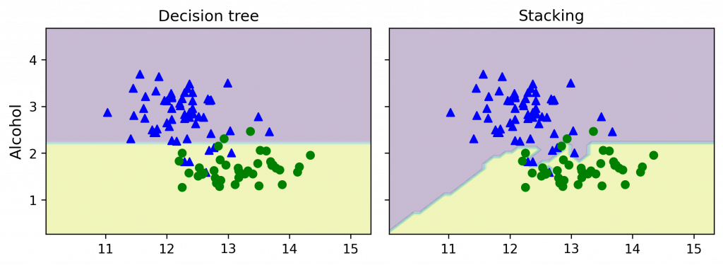

結論：

Bagging：降低模型 Variance（多數決 → 降低預測不準度）
Boosting：降低模型 Bias（矯正錯誤分類的偏差）
Stacking：強化 predictive force（y 作為 Meta-Model 的 x）
.
.
.
.
.
*補充 1. 多數投票法範例的決策邊界圖

sc = StandardScaler()
X_train_std = sc.fit_transform(X_train)

import numpy as np
from itertools import product

x_min, x_max = X_train_std[:, 0].min() - 1, X_train_std[:, 0].max() + 1
y_min, y_max = X_train_std[:, 1].min() - 1, X_train_std[:, 1].max() + 1

xx, yy = np.meshgrid(np.arange(x_min, x_max, 0.1),
                     np.arange(y_min, y_max, 0.1)
                    )

f, axarr = plt.subplots(nrows=2, ncols=2, 
                        sharex='col', 
                        sharey='row', 
                        figsize=(7, 5))

for idx, clf, tt in zip(product([0, 1], [0, 1]), all_clf, labels):
    clf.fit(X_train_std, y_train)
    
    Z = clf.predict(np.c_[xx.ravel(), yy.ravel()])
    Z = Z.reshape(xx.shape)

    axarr[idx[0], idx[1]].contourf(xx, yy, Z, alpha=0.3)
    
    axarr[idx[0], idx[1]].scatter(X_train_std[y_train==0, 0], 
                                  X_train_std[y_train==0, 1], 
                                  c='blue', 
                                  marker='^',
                                  s=50)
    
    axarr[idx[0], idx[1]].scatter(X_train_std[y_train==1, 0], 
                                  X_train_std[y_train==1, 1], 
                                  c='green', 
                                  marker='o',
                                  s=50)
    
    axarr[idx[0], idx[1]].set_title(tt)

plt.text(-3.5, -5., 
         s='Sepal width [standardized]', 
         ha='center', va='center', fontsize=12)
plt.text(-12.5, 4.5, 
         s='Petal length [standardized]', 
         ha='center', va='center', 
         fontsize=12, rotation=90)
plt.show()

*補充 2. 袋裝法範例的決策邊界圖

import numpy as np
import matplotlib.pyplot as plt

x_min = X_train[:, 0].min() - 1
x_max = X_train[:, 0].max() + 1
y_min = X_train[:, 1].min() - 1
y_max = X_train[:, 1].max() + 1

xx, yy = np.meshgrid(np.arange(x_min, x_max, 0.1),
                     np.arange(y_min, y_max, 0.1))

f, axarr = plt.subplots(nrows=1, ncols=2, 
                        sharex='col', 
                        sharey='row', 
                        figsize=(8, 3))


for idx, clf, tt in zip([0, 1],
                        [tree, bag],
                        ['Decision tree', 'Bagging']):
    clf.fit(X_train, y_train)

    Z = clf.predict(np.c_[xx.ravel(), yy.ravel()])
    Z = Z.reshape(xx.shape)

    axarr[idx].contourf(xx, yy, Z, alpha=0.3)
    axarr[idx].scatter(X_train[y_train == 0, 0],
                       X_train[y_train == 0, 1],
                       c='blue', marker='^')

    axarr[idx].scatter(X_train[y_train == 1, 0],
                       X_train[y_train == 1, 1],
                       c='green', marker='o')

    axarr[idx].set_title(tt)

axarr[0].set_ylabel('Alcohol', fontsize=12)
plt.tight_layout()
plt.show()

*補充 3. 強化法範例的決策邊界圖

import numpy as np
import matplotlib.pyplot as plt

x_min, x_max = X_train[:, 0].min() - 1, X_train[:, 0].max() + 1
y_min, y_max = X_train[:, 1].min() - 1, X_train[:, 1].max() + 1

xx, yy = np.meshgrid(np.arange(x_min, x_max, 0.1),
                     np.arange(y_min, y_max, 0.1))

f, axarr = plt.subplots(nrows=1, ncols=2, 
                        sharex='col', 
                        sharey='row', 
                        figsize=(8, 3))


for idx, clf, tt in zip([0, 1],
                        [tree, ada],
                        ['Decision tree', 'AdaBoost']):
    clf.fit(X_train, y_train)

    Z = clf.predict(np.c_[xx.ravel(), yy.ravel()])
    Z = Z.reshape(xx.shape)

    axarr[idx].contourf(xx, yy, Z, alpha=0.3)
    axarr[idx].scatter(X_train[y_train == 0, 0],
                       X_train[y_train == 0, 1],
                       c='blue', marker='^')

    axarr[idx].scatter(X_train[y_train == 1, 0],
                       X_train[y_train == 1, 1],
                       c='green', marker='o')

    axarr[idx].set_title(tt)

axarr[0].set_ylabel('Alcohol', fontsize=12)
plt.tight_layout()
plt.show()

*補充 4. 黏合法範例的決策邊界圖

import numpy as np
import matplotlib.pyplot as plt

x_min, x_max = X_train[:, 0].min() - 1, X_train[:, 0].max() + 1
y_min, y_max = X_train[:, 1].min() - 1, X_train[:, 1].max() + 1

xx, yy = np.meshgrid(np.arange(x_min, x_max, 0.1),
                     np.arange(y_min, y_max, 0.1))

f, axarr = plt.subplots(nrows=1, ncols=2, 
                        sharex='col', 
                        sharey='row', 
                        figsize=(8, 3))


for idx, clf, tt in zip([0, 1, 2],
                        [tree, stk],
                        ['Decision tree', 'Stacking']):
    clf.fit(X_train, y_train)

    Z = clf.predict(np.c_[xx.ravel(), yy.ravel()])
    Z = Z.reshape(xx.shape)

    axarr[idx].contourf(xx, yy, Z, alpha=0.3)
    axarr[idx].scatter(X_train[y_train == 0, 0],
                       X_train[y_train == 0, 1],
                       c='blue', marker='^')

    axarr[idx].scatter(X_train[y_train == 1, 0],
                       X_train[y_train == 1, 1],
                       c='green', marker='o')

    axarr[idx].set_title(tt)

axarr[0].set_ylabel('Alcohol', fontsize=12)

plt.tight_layout()
plt.show()

直播研討會

{{ item.channelVendor }} {{ item.webinarstarted }} |

直播中

尚未有邦友留言

立即登入留言

15th鐵人賽 13th鐵人賽 14th鐵人賽 12th鐵人賽 11th鐵人賽鐵人賽 2019鐵人賽 2018鐵人賽 javascript 2017鐵人賽 python windows php c# windows server linux css react 程式設計 vue.js

IT邦幫忙