我會先從研究nanoGPT開始的一個重要原因是因為他的作者Andrej Karpathy。他不僅對OpenAI和特斯拉的人工智慧成果有重要的影響,而且也是深度學習社區的重要人物。最重要的是他能夠清晰、詳細地解釋他的思維方式,並且經常用自己的理解簡化複雜的模型而後復現(如GPT或LLama2)。這種方法不僅使這些複雜的模型變得更容易理解,而且也有助於不熟悉的人去理解一些方法被使用的原因。我認為Karpathy的開源專案,如nanoGPT與baby LLama2,對於像我這樣想要深入了解這些先進技術的人來說,會是一個很好的起點。
本文內容與程式碼摘自影片 Let's build GPT: from scratch, in code, spelled out.
本文使用程式碼來自原作者的colab
不知道什麼是 N-gram Language Model 的話可以先參考文章 自然语言处理中N-Gram模型介绍
簡而言之,N-gram Language Model 是一種用統計學來建構語言模型的方法。它根據已知的文字來計算接下來辭典中所有單字出現的概率。例如,在 Bigram Language Model (N=2) 中,模型會看輸入的一個單字,然後預測接下來的下一個單字可能是什麼。(依據輸入的單字計算出字典中每個單字出現的機率,然後選擇機率最高的那個。)
如果是 10-gram Language Model (N=10),模型會看前面的9個文字,然後預測下一個文字可能是什麼。
不過要注意的是,真正傳統意義上的N-gram Language Model用的是統計方法建立語言模型,而這邊的 Bigram Language Model 是使用 NN 的方法來建立語言模型。GPT的目的其實就是在用深度學習的大模型來打造一個語言模型。
下載shakespeare dataset
# We always start with a dataset to train on. Let's download the tiny shakespeare dataset
!wget https://raw.githubusercontent.com/karpathy/char-rnn/master/data/tinyshakespeare/input.txt
讀取資料集,印出細節
# read it in to inspect it
with open('input.txt', 'r', encoding='utf-8') as f:
    text = f.read()
print("length of dataset in characters: ", len(text))
length of dataset in characters: 1115394
印出文章中所有用到的字元(字典),與字典長度
# here are all the unique characters that occur in this text
chars = sorted(list(set(text)))
vocab_size = len(chars)
print(''.join(chars))
print(vocab_size)
!$&',-.3:;?ABCDEFGHIJKLMNOPQRSTUVWXYZabcdefghijklmnopqrstuvwxyz
65
encode與decode字串(charactor level 的 token)
# create a mapping from characters to integers
stoi = { ch:i for i,ch in enumerate(chars) }
itos = { i:ch for i,ch in enumerate(chars) }
encode = lambda s: [stoi[c] for c in s] # encoder: take a string, output a list of integers
decode = lambda l: ''.join([itos[i] for i in l]) # decoder: take a list of integers, output a string

print(encode("hii there"))
print(decode(encode("hii there")))
[46, 47, 47, 1, 58, 46, 43, 56, 43]
hii there
使用前 90% 當 training data,後 10% 當 val data
# Let's now split up the data into train and validation sets
n = int(0.9*len(data)) # first 90% will be train, rest val
train_data = data[:n]
val_data = data[n:]
印出訓練時的data(x)跟label(y)看一下
x = train_data[:block_size]
y = train_data[1:block_size+1]
for t in range(block_size):
    context = x[:t+1]
    target = y[t]
    print(f"when input is {context} the target: {target}")
when input is tensor([18]) the target: 47
when input is tensor([18, 47]) the target: 56
when input is tensor([18, 47, 56]) the target: 57
when input is tensor([18, 47, 56, 57]) the target: 58
when input is tensor([18, 47, 56, 57, 58]) the target: 1
when input is tensor([18, 47, 56, 57, 58, 1]) the target: 15
when input is tensor([18, 47, 56, 57, 58, 1, 15]) the target: 47
when input is tensor([18, 47, 56, 57, 58, 1, 15, 47]) the target: 58
!$&',-.3:;?ABCDEFGHIJKLMNOPQRSTUVWXYZabcdefghijklmnopqrstuvwxyz
import torch
import torch.nn as nn
from torch.nn import functional as F
torch.manual_seed(1337)

class BigramLanguageModel(nn.Module):

    def __init__(self, vocab_size):
        super().__init__()
        # each token directly reads off the logits for the next token from a lookup table
        self.token_embedding_table = nn.Embedding(vocab_size, vocab_size)

    def forward(self, idx, targets=None):

        # idx and targets are both (B,T) tensor of integers
        logits = self.token_embedding_table(idx) # (B,T,C)

        if targets is None:
            loss = None
        else:
            B, T, C = logits.shape
            logits = logits.view(B*T, C)
            targets = targets.view(B*T)
            loss = F.cross_entropy(logits, targets)

        return logits, loss

    def generate(self, idx, max_new_tokens):
        # idx is (B, T) array of indices in the current context
        for _ in range(max_new_tokens):
            # get the predictions
            logits, loss = self(idx)
            # focus only on the last time step
            logits = logits[:, -1, :] # becomes (B, C)
            # apply softmax to get probabilities
            probs = F.softmax(logits, dim=-1) # (B, C)
            # sample from the distribution
            idx_next = torch.multinomial(probs, num_samples=1) # (B, 1)
            # append sampled index to the running sequence
            idx = torch.cat((idx, idx_next), dim=1) # (B, T+1)
        return idx
定義get_batch(),device, m(model)
torch.manual_seed(1337)
batch_size = 4 # how many independent sequences will we process in parallel?
block_size = 32 # what is the maximum context length for predictions?

def get_batch(split):
    # generate a small batch of data of inputs x and targets y
    data = train_data if split == 'train' else val_data
    ix = torch.randint(len(data) - block_size, (batch_size,))
    x = torch.stack([data[i:i+block_size] for i in ix])
    y = torch.stack([data[i+1:i+block_size+1] for i in ix])
    return x, y

xb, yb = get_batch('train')
print('inputs:')
print(xb.shape)
print(xb)
print('targets:')
print(yb.shape)
print(yb)

# create a PyTorch optimizer
optimizer = torch.optim.AdamW(m.parameters(), lr=1e-3)

# get device
device = torch.device('cuda' if torch.cuda.is_available() else 'cpu')

# create model
m = BigramLanguageModel(vocab_size).to(device)
logits, loss = m(xb.to(device), yb.to(device))
print(logits.shape)
print(loss)
print(decode(m.generate(idx = torch.zeros((1, 1), dtype=torch.long).to(device), max_new_tokens=100)[0].tolist()))
可以先印出訓練前的預測結果看看,是完全的亂碼。
print(decode(m.generate(idx = torch.zeros((1, 1), dtype=torch.long).cuda(), max_new_tokens=500)[0].tolist()))
開始訓練
from tqdm import tqdm
for steps in tqdm(range(1000000)): # increase number of steps for good results...
    # sample a batch of data
    xb, yb = get_batch('train')

    # evaluate the loss
    logits, loss = m(xb.to(device), yb.to(device))
    optimizer.zero_grad(set_to_none=True)
    loss.backward()
    optimizer.step()
印出訓練後的預測結果
print(decode(m.generate(idx = torch.zeros((1, 1), dtype=torch.long).cuda(), max_new_tokens=500)[0].tolist()))
這裡使用shakespeare的文章集來訓練一個Bigram Language Model,可以看出學習前生成的結果都是亂碼,但是在訓練後,輸出是可以看出有一個模仿shakespeare的雛型並非純粹的亂碼,雖然結果不好(畢竟只是Bigram,使用的N太小,而且用的token又是字元)。不過之後的修改都會基於這個Bigram Language Model,一步一步改進最終做出nanoGPT。
補充說明:GPT的架構是Transformer中的decoder,因此這邊在思考 Attention 的時候,講的是Self-Attention,並且輸入都是有順序的,前面的node不能參考後面的資訊:
t1 時的 input = [x1], weight = [w11] ; out1 = x1w11
t2 時的 input = [x1, x2], weight = [w21, w22] ; out2 = x1w21 + x2w22
t3 時的 input = [x1, x2, x3], weight = [w31, w32, w33] ; out3 = x1we1 + x2w32 + x3w33
如何計算出各個時間點 t 之下對應的 out (weighted aggregation),是這邊要探討的內容。
初始化參數
import torch
# consider the following toy example:
torch.manual_seed(1337)
B,T,C = 4,8,2 # batch, time, channels
x = torch.randn(B,T,C)
x.shape
如果想要循序計算weighted aggregation時,最直接的作法
這邊使用torch.mean(...)來代替weight,假設x內的所有element weight均等。
# We want x[b,t] = mean_{i<=t} x[b,i]
xbow = torch.zeros((B,T,C))
for b in range(B):
    for t in range(T):
        xprev = x[b,:t+1] # (t,C)
        xbow[b,t] = torch.mean(xprev, 0)
改成用矩陣相乘來實做 weighted aggregation
計算結果完全是等價,但因為使用矩陣相乘,明顯更適合平行優化;缺點是完全失去順序的概念。
# version 2: using matrix multiply for a weighted aggregation
wei = torch.tril(torch.ones(T, T))
wei = wei / wei.sum(1, keepdim=True)
xbow2 = wei @ x # (B, T, T) @ (B, T, C) ----> (B, T, C)
print("xbow==xbow2 ? "+str(torch.allclose(xbow, xbow2)))
### True
使用 Softmax 將 分數(wei) 轉換成 權重(加總等於1)
masked self-attention的雛型
# version 3: use Softmax
tril = torch.tril(torch.ones(T, T))
wei = torch.zeros((T,T))
wei = wei.masked_fill(tril == 0, float('-inf'))
wei = F.softmax(wei, dim=-1)
xbow3 = wei @ x
print("xbow==xbow3 ? "+str(torch.allclose(xbow, xbow3)))
### True
輸入print(wei[0])將轉換後的權重印出來,可以看到masked self-attention的權重中,每一個node都是自己與先前所有node的weighted sum,未來的node都被masked掉。
在t1時,只有第一個權重值是1,其後全部都是0
在t2時,只有第一跟第二個權重有值,其後全部都是0
tensor([
    [1.0000, 0.0000, 0.0000, 0.0000, 0.0000, 0.0000, 0.0000, 0.0000],
    [0.1574, 0.8426, 0.0000, 0.0000, 0.0000, 0.0000, 0.0000, 0.0000],
    [0.2088, 0.1646, 0.6266, 0.0000, 0.0000, 0.0000, 0.0000, 0.0000],
    [0.5792, 0.1187, 0.1889, 0.1131, 0.0000, 0.0000, 0.0000, 0.0000],
    [0.0294, 0.1052, 0.0469, 0.0276, 0.7909, 0.0000, 0.0000, 0.0000],
    [0.0176, 0.2689, 0.0215, 0.0089, 0.6812, 0.0019, 0.0000, 0.0000],
    [0.1691, 0.4066, 0.0438, 0.0416, 0.1048, 0.2012, 0.0329, 0.0000],
    [0.0210, 0.0843, 0.0555, 0.2297, 0.0573, 0.0709, 0.2423, 0.2391]
], grad_fn=<SelectBackward0>)
完成Masked Self-Attention
query, key, value,並加上一層nn.Linear()做映射wei = wei.masked_fill(tril == 0, float('-inf')) 拿掉就變回正常的 attention
self-attention:query, key, value來源都是x
cross-attention:query輸入為x,key,value輸入為‵y‵# version 4: self-attention!
torch.manual_seed(1337)
B,T,C = 4,8,32 # batch, time, channels
x = torch.randn(B,T,C)
# let's see a single Head perform self-attention
head_size = 16
key = nn.Linear(C, head_size, bias=False)
query = nn.Linear(C, head_size, bias=False)
value = nn.Linear(C, head_size, bias=False)
k = key(x) # (B, T, 16)
q = query(x) # (B, T, 16)
wei = q @ k.transpose(-2, -1) # (B, T, 16) @ (B, 16, T) ---> (B, T, T)
tril = torch.tril(torch.ones(T, T))
#wei = torch.zeros((T,T))
wei = wei.masked_fill(tril == 0, float('-inf'))
wei = F.softmax(wei, dim=-1)
v = value(x)
out = wei @ v
Attention 機制是沒有順序概念的
Attention 機制允許模型在序列的元素之間共享信息,但是這個過程本身是不考慮元素的順序的。換句話說,注意力機制本身不知道序列中的元素的順序,因此它會以相同的方式處理序列中的所有元素,無論它們的位置如何。這是一個問題,因為許多序列數據(例如自然語言文本)中的元素的順序是非常重要的。
Positional Encoding
為了解決這個問題,可以使用 "Positional Encoding"。這是一種將位置信息編碼到序列的元素中的方法。具體來說,我們可以為序列中的每個位置生成一個向量,然後將這個向量添加到該位置的元素的表示中。這樣,模型就可以根據元素的位置來處理它們。
因此,"Positional Encoding" 是一個讓Attention模型能夠考慮到序列中元素的順序的方法,這對於許多自然語言處理任務是至關重要的。
batch element之間是獨立的
(B, T, C) @ (B, C, T) -> (B, T, T),torch的矩陣相乘操作會在B個平行空間中將TxC矩陣與CxT矩陣做相乘,因此batch element之間是完全獨立的。
def forward(self, x):
    B,T,C = x.shape
    k = self.key(x)   # (B,T,C)
    q = self.query(x) # (B,T,C)
    # compute attention scores ("affinities")
    wei = q @ k.transpose(-2,-1) * C**-0.5 # (B, T, C) @ (B, C, T) -> (B, T, T)
    ...
Encoder & Decoder Block
Encoder: 會移除wei = wei.masked_fill(tril == 0, float('-inf')) 這一行,每個node都可以取得其後面的node的資訊。Decoder: 則會加入這個限制,tril 是一個下三角矩陣,用於 mask 掉注意力權重矩陣的一部分。這種注意力機制只允許模型考慮當前位置或之前的位置,而不允許考慮未來的位置。Weight Normalization for Softmax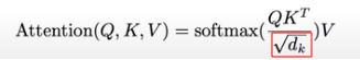
= 程式中的
head_size
將weight正規化令var(weight)=1,因為weight將會作為softmax的輸入,若head_size很大導致weight的值域太大的話,會導致softmax(weight)的值變得很極端。
softmax的特性:大的值經過softmax會放大,小的值經過softmax會縮小;如果輸入的值彼此間差距太大,很容易會造成最後只有最大的值被放大到接近1,其餘值都被縮小成無限接近0。
import torch
print(torch.softmax(torch.tensor([0.1, -0.2, 0.3, -0.2, 0.5]), dim=-1))
### tensor([0.1925, 0.1426, 0.2351, 0.1426, 0.2872])
print(torch.softmax(torch.tensor([0.1, -0.2, 0.3, -0.2, 0.5])*8, dim=-1))
### tensor([0.0326, 0.0030, 0.1615, 0.0030, 0.8000]
nn.Module.register_buffer('tril', ...):在宣告變數時向nn.Module註冊tensor變數tril,確保save/load時都會處理tril的值,但在optimize的時候不作更新。class Head(nn.Module):
""" one head of self-attention """
def __init__(self, head_size):
super().__init__()
self.key = nn.Linear(n_embd, head_size, bias=False)
self.query = nn.Linear(n_embd, head_size, bias=False)
self.value = nn.Linear(n_embd, head_size, bias=False)
self.register_buffer('tril', torch.tril(torch.ones(block_size, block_size)))
self.dropout = nn.Dropout(dropout)
def forward(self, x):
B,T,C = x.shape
k = self.key(x) # (B,T,C)
q = self.query(x) # (B,T,C)
# compute attention scores ("affinities")
wei = q @ k.transpose(-2,-1) * C**-0.5 # (B, T, C) @ (B, C, T) -> (B, T, T)
wei = wei.masked_fill(self.tril[:T, :T] == 0, float('-inf')) # (B, T, T)
wei = F.softmax(wei, dim=-1) # (B, T, T)
wei = self.dropout(wei)
# perform the weighted aggregation of the values
v = self.value(x) # (B,T,C)
out = wei @ v # (B, T, T) @ (B, T, C) -> (B, T, C)
return out
從forward()定義可以看出: Multi-head attetion只是同時使用了 N 個 Attention 平行處理輸入x並且將輸出結果concat起來,N 個 Attention 模組之前是完全獨立的。
class MultiHeadAttention(nn.Module):
    """ multiple heads of self-attention in parallel """

    def __init__(self, num_heads, head_size):
        super().__init__()
        self.heads = nn.ModuleList([Head(head_size) for _ in range(num_heads)])
        self.proj = nn.Linear(n_embd, n_embd)
        self.dropout = nn.Dropout(dropout)

    def forward(self, x):
        out = torch.cat([h(x) for h in self.heads], dim=-1)
        out = self.dropout(self.proj(out))
        return out
用於將前一層的Multi-head attention的結果做一個整合。
class FeedFoward(nn.Module):
    """ a simple linear layer followed by a non-linearity """

    def __init__(self, n_embd):
        super().__init__()
        self.net = nn.Sequential(
            nn.Linear(n_embd, 4 * n_embd),
            nn.ReLU(),
            nn.Linear(4 * n_embd, n_embd),
            nn.Dropout(dropout),
        )

    def forward(self, x):
        return self.net(x)
作者是把之前自己寫的BatchNorm稍微修改,變成了LayerNorm。有時間的話,這邊可以自己練習一下,把LayerNorm的程式碼再修改回BatchNorm。
class LayerNorm1d: # (used to be BatchNorm1d)

  def __init__(self, dim, eps=1e-5, momentum=0.1):
    self.eps = eps
    self.gamma = torch.ones(dim)
    self.beta = torch.zeros(dim)

  def __call__(self, x):
    # calculate the forward pass
    xmean = x.mean(1, keepdim=True) # batch mean
    xvar = x.var(1, keepdim=True) # batch variance
    xhat = (x - xmean) / torch.sqrt(xvar + self.eps) # normalize to unit variance
    self.out = self.gamma * xhat + self.beta
    return self.out

  def parameters(self):
    return [self.gamma, self.beta]


 iThome鐵人賽