(聲明:以下內容都是在網路上整理並修改的,真正我原創的內容並不多,我主要只是搬運工)
原始的論文連結: Deep Residual Learning for Image Recognition
程式碼跟原理一起介紹的Blog: DIVE INTO DEEP LEARNING:ResNet
我這邊除了原本的基礎外,會在其他地方做點進階。
ResNet(Residual Network)是一種深度學習架構,專為解決深度神經網絡中的梯度消失和梯度爆炸問題而設計。以下是對其主要原理和算法的詳細介紹:
ResNet(殘差網絡)主要解決了深度神經網絡中的梯度消失(或梯度爆炸)問題,這使得網絡能夠更容易地訓練更深的結構。在傳統的深度網絡中,隨著層數的增加,模型的性能往往會達到一個瓶頸,甚至會變差。這是因為梯度在反向傳播過程中會變得非常小(梯度消失)或非常大(梯度爆炸),導致網絡難以學習。
ResNet 通過引入“殘差塊”(Residual Blocks)來解決這個問題。每個殘差塊都包含一個“捷徑連接”(Shortcut Connection),也就是一個將輸入直接連接到輸出的路徑。這樣,即使網絡的其他部分在訓練過程中出現梯度消失或梯度爆炸,捷徑連接也能保證梯度能夠順利地反向傳播。
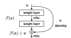
具體來說,傳統的深度網絡試圖學習一個目標函數 $H(x)$,而 ResNet 則試圖學習這個函數與輸入 $x$ 之間的殘差$F(x)=H(x)−x$。然後它將這個殘差加回輸入,得到$H(x)=F(x)+x$。
這種設計使得 ResNet 能夠有效地訓練非常深的網絡(數百層或更多),並在多個視覺識別任務上達到先進的性能。
殘差學習(Residual Learning): ResNet 的核心思想是學習輸入和輸出之間的殘差映射,而不是直接學習輸出。換句話說,給定一個輸入 $x$ 和一個輸出 $F(x)=H(x)-x$ ,ResNet 會學習
$F(x)=H(x)-x$,然後將$F(x)$加回$x$ 以得到最終輸出。
捷徑連接(Shortcut Connections): 每個殘差塊都包含一個捷徑連接,這是一個將輸入直接連接到輸出的路徑。這確保了梯度可以直接通過這些連接反向傳播,從而緩解梯度消失問題。
堆疊殘差塊(Stacking Residual Blocks): ResNet 由多個這種殘差塊組成,每個塊內部都可能包含多個卷積層、激活函數和正則化層。
輸入預處理: 對輸入數據進行必要的預處理,如縮放、中心化等。
初始卷積層: 通常會有一個初始的卷積層來捕獲低級特徵。
殘差塊組成: 接著是多個殘差塊,每個殘差塊都有一個或多個卷積層和一個捷徑連接。
激活函數: 每個卷積層後通常會跟一個激活函數,如 ReLU。
合併: 在殘差塊的末尾,捷徑連接的輸出和卷積層的輸出會相加。
全連接層和輸出: 在所有殘差塊之後,通常會有一個或多個全連接層,最後是輸出層。
損失函數和優化: 使用適當的損失函數和優化算法來訓練網絡。
反向傳播和權重更新: 在訓練過程中,使用反向傳播算法來更新網絡權重。
通過這種設計,ResNet 能夠有效地訓練非常深的網絡,並在各種視覺識別任務上達到或超越當前的最佳性能。
下圖為34層的網路示意圖: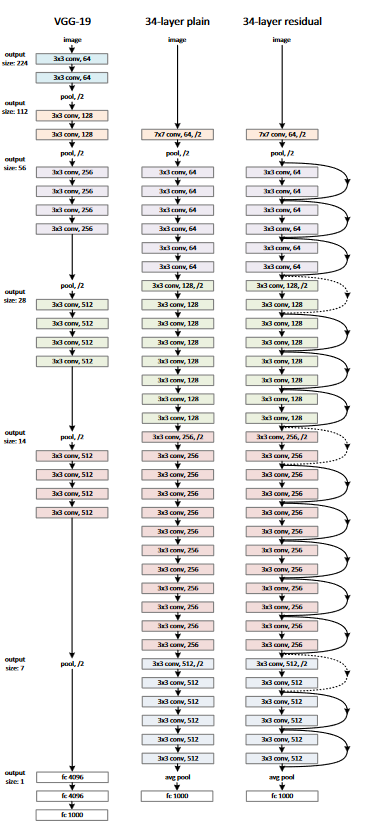
import numpy as np
import torch
import torch.nn as nn
from torchvision import datasets
from torchvision import transforms
from torch.utils.data.sampler import SubsetRandomSampler


# 預設成使用gpu計算
device = torch.device('cuda' if torch.cuda.is_available() else 'cpu')
這邊是使用CIFAR-10資料集
這邊首先定義data_loader這個函數,該函數根據參數返回訓練或測試的資料。
在深度學習項目中標準化資料始終是一個很好的做法,這可讓訓練更快、更容易收斂。為此,我們normalize使用資料集中每個RGB 色版(0~255)(紅色R、綠色G和藍色B)的平均值和標準差來定義變量。這些可以手動計算,但也可以在線獲取。我們在 transform 這個函數中調整數據大小,將其轉換為張量,然後對其進行標準化。
data loaders:這資料加載器的設計允許我們循環的迭代下載新資料,資料在迭代時加載,而不是在啟動時一次性全部加載到 RAM 中。 這在處理大約百萬張圖像的大型資料集時非常有幫助。
根據test這參數,我們要么加載訓練集 (if test=False) 分割,要么加載測試集(if test=True) 分割。對於訓練集,資料會被隨機分為訓練集和驗證集(0.9:0.1)。
# 導入所需的庫
from torchvision import datasets, transforms
import torch
import numpy as np
from torch.utils.data.sampler import SubsetRandomSampler
# 定義一個函數來加載數據
def data_loader(data_dir,
                batch_size,
                random_seed=42,
                valid_size=0.1,
                shuffle=True,
                test=False):
    # 正規化數據集
    normalize = transforms.Normalize(
        mean=[0.4914, 0.4822, 0.4465],
        std=[0.2023, 0.1994, 0.2010],
    )

    # define transforms 定義數據轉換
    transform = transforms.Compose([
            transforms.Resize((224,224)), # 調整圖像大小
            transforms.ToTensor(), # 轉換為張量
            normalize, # 正規化
    ])
     # 如果是測試集
    if test:
        dataset = datasets.CIFAR10(
          root=data_dir, train=False,
          download=True, transform=transform,
        )

        data_loader = torch.utils.data.DataLoader(
            dataset, batch_size=batch_size, shuffle=shuffle
        )

        return data_loader

    # load the dataset  加載訓練集
    dataset = datasets.CIFAR10(root=data_dir, train=True, download=True, transform=transform)

    num_train = len(dataset)
    indices = list(range(num_train))
    split = int(np.floor(valid_size * num_train))
    # 是否打亂數據
    if shuffle:
        np.random.seed(random_seed)
        np.random.shuffle(indices)
    # 分割訓練集和驗證集
    train_idx, valid_idx = indices[split:], indices[:split]

    train_sampler = SubsetRandomSampler(train_idx)
    valid_sampler = SubsetRandomSampler(valid_idx)
    # 創建訓練和驗證數據加載器
    train_loader = torch.utils.data.DataLoader(
        dataset, batch_size=batch_size, sampler=train_sampler)

    valid_loader = torch.utils.data.DataLoader(
        dataset, batch_size=batch_size, sampler=valid_sampler)

    return (train_loader, valid_loader)


# CIFAR10 dataset 使用函數來加載CIFAR10數據集
train_loader, valid_loader = data_loader(data_dir='./data',
                                         batch_size=64)

test_loader = data_loader(data_dir='./data',
                              batch_size=64,
                              test=True)
在繼續構建殘差層和 ResNet 之前,我們首先研究並理解 PyTorch 中如何定義神經網絡:
nn.Module提供了用於創建自定義模型的樣板以及一些有助於訓練模型的必要功能。這就是為什麼每個自定義模型都傾向於繼承自nn.Module
每個自定義模型內部都有兩個主要功能。
第一個是初始化函數 init:我們在其中定義將使用的各個層
第二個是函數forward:輸入會跟此函數上設定的功能處理輸入的值
現在介紹 PyTorch 中可用的對我們有用的不同類型的層:
# 定義ResidualBlock類,繼承自nn.Module
class ResidualBlock(nn.Module):
    # 初始化函數
    def __init__(self, in_channels, out_channels, stride = 1, downsample = None):
        # 調用父類的初始化函數
        super(ResidualBlock, self).__init__()
        # 第一個卷積層,包括卷積、批量正規化和ReLU激活
        self.conv1 = nn.Sequential(
                        nn.Conv2d(in_channels, out_channels, kernel_size = 3, stride = stride, padding = 1),
                        nn.BatchNorm2d(out_channels),
                        nn.ReLU())
        # 第二個卷積層,包括卷積和批量正規化
        self.conv2 = nn.Sequential(
                        nn.Conv2d(out_channels, out_channels, kernel_size = 3, stride = 1, padding = 1),
                        nn.BatchNorm2d(out_channels))
        # 下採樣層,用於調整殘差的維度
        self.downsample = downsample
        # ReLU激活函數
        self.relu = nn.ReLU()
        # 輸出通道數
        self.out_channels = out_channels
    # 前向傳播函數
    def forward(self, x):
        # 保存輸入作為殘差
        residual = x
        # 通過第一個卷積層
        out = self.conv1(x)
        out = self.conv2(out)# 通過第二個卷積層
        # 如果有下採樣,對殘差進行下採樣
        if self.downsample:
            residual = self.downsample(x)
        # 將輸出和殘差相加
        out += residual
        # 通過ReLU激活函數
        out = self.relu(out)
        return out
在設定好 ResidualBlock後,就可以構建 ResNet了。
請注意,該架構中有三個塊,分別包含 3、4、6 和 3 層。
這邊創建一個輔助函數_make_layer以完成ResNet的構建。該函數將各層與殘差塊逐個添加。
# 定義ResNet類,繼承自nn.Module
class ResNet(nn.Module):
    # 初始化函數
    def __init__(self, block, layers, num_classes = 10):
        # 調用父類的初始化函數
        super(ResNet, self).__init__()
        # 初始化輸入通道數
        self.inplanes = 64
        # 第一個卷積層,包括卷積、批量正規化和ReLU激活
        self.conv1 = nn.Sequential(
                        nn.Conv2d(3, 64, kernel_size = 7, stride = 2, padding = 3),
                        nn.BatchNorm2d(64),
                        nn.ReLU())
        # 最大池化層
        self.maxpool = nn.MaxPool2d(kernel_size = 3, stride = 2, padding = 1)
        # 創建四個殘差層
        self.layer0 = self._make_layer(block, 64, layers[0], stride = 1)
        self.layer1 = self._make_layer(block, 128, layers[1], stride = 2)
        self.layer2 = self._make_layer(block, 256, layers[2], stride = 2)
        self.layer3 = self._make_layer(block, 512, layers[3], stride = 2)
        # 平均池化層
        self.avgpool = nn.AvgPool2d(7, stride=1)
        # 全連接層
        self.fc = nn.Linear(512, num_classes)
    # 創建殘差層的函數
    def _make_layer(self, block, planes, blocks, stride=1):
        downsample = None
        # 判斷是否需要下採樣
        if stride != 1 or self.inplanes != planes:

            downsample = nn.Sequential(
                nn.Conv2d(self.inplanes, planes, kernel_size=1, stride=stride),
                nn.BatchNorm2d(planes),
            )
        # 初始化殘差塊列表
        layers = []
        # 添加第一個殘差塊,可能包含下採樣
        layers.append(block(self.inplanes, planes, stride, downsample))
        # 更新輸入通道數
        self.inplanes = planes
        # 添加其他殘差塊
        for i in range(1, blocks):
            layers.append(block(self.inplanes, planes))
        # 返回殘差層
        return nn.Sequential(*layers)

    # 前向傳播函數
    def forward(self, x):
        x = self.conv1(x)
        x = self.maxpool(x)
        x = self.layer0(x)
        x = self.layer1(x)
        x = self.layer2(x)
        x = self.layer3(x)

        x = self.avgpool(x)
        x = x.view(x.size(0), -1)
        x = self.fc(x)

        return x
這邊推薦每個人在模型中嘗試各種超參數的不同值,或使用 optuna這類的套件自動調整超參數。
超參數包括定義輪數、批量大小、學習率、損失函數以及優化器。
訓練過程如下:
# 設定參數
num_classes = 10 # 分類數量
num_epochs = 20 # 訓練迭代次數
batch_size = 16 # 批次大小
learning_rate = 0.01 # 學習率

# 初始化模型並將其移至設備(這邊是GPU)
model = ResNet(ResidualBlock, [3, 4, 6, 3]).to(device)

# Loss and optimizer定義損失函數和優化器
criterion = nn.CrossEntropyLoss() # 交叉熵損失
optimizer = torch.optim.SGD(model.parameters(), lr=learning_rate, weight_decay = 0.001, momentum = 0.9)# 隨機梯度下降優化器

# Train the model 訓練模型
total_step = len(train_loader)# 訓練數據的批次數
# 引入垃圾回收模塊
import gc
# 開始訓練迴圈
for epoch in range(num_epochs):
    for i, (images, labels) in enumerate(train_loader):
        # 將張量移至配置的設備
        images = images.to(device)
        labels = labels.to(device)

        # 前向傳播
        outputs = model(images)
        loss = criterion(outputs, labels)

        # 反向傳播和優化
        optimizer.zero_grad()# 清空梯度
        loss.backward()# 反向傳播
        optimizer.step()# 更新參數
        del images, labels, outputs# 釋放不必要的記憶體
        torch.cuda.empty_cache()# 清空CUDA緩存
        gc.collect() # 垃圾回收
    # 輸出每個epoch的損失
    print ('Epoch [{}/{}], Loss: {:.4f}'
                   .format(epoch+1, num_epochs, loss.item()))

    # 驗證模型
    with torch.no_grad():# 不計算梯度
        correct = 0
        total = 0
        for images, labels in valid_loader:
            images = images.to(device)
            labels = labels.to(device)
            outputs = model(images)
            _, predicted = torch.max(outputs.data, 1)
            total += labels.size(0)
            correct += (predicted == labels).sum().item()
            del images, labels, outputs# 釋放不必要的記憶體
        # 輸出驗證集上的準確率
        print('Accuracy of the network on the {} validation images: {} %'.format(5000, 100 * correct / total))
Epoch [1/20], Loss: 2.5937
Accuracy of the network on the 5000 validation images: 58.32 %
Epoch [2/20], Loss: 0.4738
Accuracy of the network on the 5000 validation images: 72.52 %
Epoch [3/20], Loss: 2.4518
Accuracy of the network on the 5000 validation images: 76.46 %
Epoch [4/20], Loss: 1.3414
Accuracy of the network on the 5000 validation images: 77.84 %
Epoch [5/20], Loss: 0.1207
Accuracy of the network on the 5000 validation images: 80.8 %
Epoch [6/20], Loss: 0.7945
Accuracy of the network on the 5000 validation images: 82.26 %
Epoch [7/20], Loss: 0.2562
Accuracy of the network on the 5000 validation images: 82.02 %
Epoch [8/20], Loss: 0.2751
Accuracy of the network on the 5000 validation images: 82.34 %
Epoch [9/20], Loss: 0.0845
Accuracy of the network on the 5000 validation images: 82.92 %
Epoch [10/20], Loss: 1.5647
Accuracy of the network on the 5000 validation images: 83.3 %
Epoch [11/20], Loss: 0.1036
Accuracy of the network on the 5000 validation images: 83.98 %
Epoch [12/20], Loss: 0.9917
Accuracy of the network on the 5000 validation images: 83.18 %
Epoch [13/20], Loss: 0.0957
Accuracy of the network on the 5000 validation images: 83.9 %
Epoch [14/20], Loss: 0.0137
Accuracy of the network on the 5000 validation images: 83.58 %
Epoch [15/20], Loss: 0.0821
Accuracy of the network on the 5000 validation images: 83.3 %
Epoch [16/20], Loss: 0.1833
Accuracy of the network on the 5000 validation images: 83.06 %
Epoch [17/20], Loss: 0.0280
Accuracy of the network on the 5000 validation images: 83.04 %
Epoch [18/20], Loss: 0.1073
Accuracy of the network on the 5000 validation images: 82.64 %
Epoch [19/20], Loss: 0.1173
Accuracy of the network on the 5000 validation images: 81.86 %
Epoch [20/20], Loss: 0.1241
Accuracy of the network on the 5000 validation images: 83.94 %
# 這邊的程式碼跟上面驗證的程式碼差別只在一個是載入驗證集(valid_loader),一個是載入測試集(test_loader)
with torch.no_grad():
    correct = 0
    total = 0
    for images, labels in test_loader:
        images = images.to(device)
        labels = labels.to(device)
        outputs = model(images)
        _, predicted = torch.max(outputs.data, 1)
        total += labels.size(0)
        correct += (predicted == labels).sum().item()
        del images, labels, outputs

    print('Accuracy of the network on the {} test images: {} %'.format(10000, 100 * correct / total))
Accuracy of the network on the 10000 test images: 83.07 %
這邊是使用官方的教學使用預訓練模型進行圖像分類
Deep residual networks pre-trained on ImageNet
import torch
model = torch.hub.load('pytorch/vision:v0.10.0', 'resnet18', pretrained=True)
# or any of these variants
# model = torch.hub.load('pytorch/vision:v0.10.0', 'resnet34', pretrained=True)
# model = torch.hub.load('pytorch/vision:v0.10.0', 'resnet50', pretrained=True)
# model = torch.hub.load('pytorch/vision:v0.10.0', 'resnet101', pretrained=True)
# model = torch.hub.load('pytorch/vision:v0.10.0', 'resnet152', pretrained=True)
model.eval()
Pytorch中所有預訓練模型都預設輸入圖像以相同的方式標準化,
即形狀為“(3 x H x W)”的 3 通道 RGB 的小批量(mini-batches)圖像,其中“H”和“W”預計至少為“224”。
圖像必須加載到“[0, 1]”範圍內,然後使用 mean = [0.485, 0.456, 0.406]和 std = [0.229, 0.224, 0.225]進行標準化。
下面是一個執行範例。
# Download an example image from the pytorch website
import urllib
url, filename = ("https://github.com/pytorch/hub/raw/master/images/dog.jpg", "dog.jpg")
try: urllib.URLopener().retrieve(url, filename)
except: urllib.request.urlretrieve(url, filename)
# sample execution (requires torchvision)
from PIL import Image
from torchvision import transforms
input_image = Image.open(filename)
preprocess = transforms.Compose([
    transforms.Resize(256),
    transforms.CenterCrop(224),
    transforms.ToTensor(),
    transforms.Normalize(mean=[0.485, 0.456, 0.406], std=[0.229, 0.224, 0.225]),
])
input_tensor = preprocess(input_image)
input_batch = input_tensor.unsqueeze(0) # create a mini-batch as expected by the model

# move the input and model to GPU for speed if available
if torch.cuda.is_available():
    input_batch = input_batch.to('cuda')
    model.to('cuda')

with torch.no_grad():
    output = model(input_batch)
# Tensor of shape 1000, with confidence scores over Imagenet's 1000 classes
print(output[0])
# The output has unnormalized scores. To get probabilities, you can run a softmax on it.
probabilities = torch.nn.functional.softmax(output[0], dim=0)
print(probabilities)
# Download ImageNet labels
!wget https://raw.githubusercontent.com/pytorch/hub/master/imagenet_classes.txt
# Read the categories
with open("imagenet_classes.txt", "r") as f:
    categories = [s.strip() for s in f.readlines()]
# Show top categories per image
top5_prob, top5_catid = torch.topk(probabilities, 5)
for i in range(top5_prob.size(0)):
    print(categories[top5_catid[i]], top5_prob[i].item())
Samoyed 0.8846220374107361
Arctic fox 0.045805152505636215
white wolf 0.044276218861341476
Pomeranian 0.005621326621621847
Great Pyrenees 0.004652002360671759
原作的連結在這:how to build a resnet from scratch with tensorflow 2 and keras
其實跟pytorch的流程是類似的,區別只有使用套件的不同。
import os
import numpy as np
import tensorflow
from tensorflow.keras import Model
from tensorflow.keras.datasets import cifar10
from tensorflow.keras.layers import Add, GlobalAveragePooling2D,\
	Dense, Flatten, Conv2D, Lambda,	Input, BatchNormalization, Activation
from tensorflow.keras.optimizers import schedules, SGD
from tensorflow.keras.callbacks import TensorBoard, ModelCheckpoint

# 定義模型配置函數
def model_configuration():
	"""
		獲取模型的配置變量。
	"""

	# 加載數據集以計算數據集大小
	(input_train, _), (_, _) = load_dataset()

	# 通用配置
	width, height, channels = 32, 32, 3
	batch_size = 128
	num_classes = 10
	validation_split = 0.1 # 根據He等人的論文,45/5
	verbose = 1
	n = 3
	init_fm_dim = 16
	shortcut_type = "identity" # or: projection

	# 數據集大小
	train_size = (1 - validation_split) * len(input_train)
	val_size = (validation_split) * len(input_train)

	# 每個 epoch 的步數取決於 batch size
	maximum_number_iterations = 64000 # 根據He等人的論文
	steps_per_epoch = tensorflow.math.floor(train_size / batch_size)
	val_steps_per_epoch = tensorflow.math.floor(val_size / batch_size)
	epochs = tensorflow.cast(tensorflow.math.floor(maximum_number_iterations / steps_per_epoch),\
		dtype=tensorflow.int64)

	# 定義損失函數
	loss = tensorflow.keras.losses.CategoricalCrossentropy(from_logits=True)

	# 根據He等人的論文配置學習率
	boundaries = [32000, 48000]
	values = [0.1, 0.01, 0.001]
	lr_schedule = schedules.PiecewiseConstantDecay(boundaries, values)

	# 設置層初始化
	initializer = tensorflow.keras.initializers.HeNormal()

	# 定義優化器
	optimizer_momentum = 0.9
	optimizer_additional_metrics = ["accuracy"]
	optimizer = SGD(learning_rate=lr_schedule, momentum=optimizer_momentum)

	# 加載Tensorboard回調函數
	tensorboard = TensorBoard(
	  log_dir=os.path.join(os.getcwd(), "logs"),
	  histogram_freq=1,
	  write_images=True
	)

	# 在每個epoch之後保存模型檢查點
	checkpoint = ModelCheckpoint(
		os.path.join(os.getcwd(), "model_checkpoint"),
		save_freq="epoch"
	)

	# 將回調函數添加到列表中
	callbacks = [
	  tensorboard,
	  checkpoint
	]

	# 創建配置字典
	config = {
		"width": width,
		"height": height,
		"dim": channels,
		"batch_size": batch_size,
		"num_classes": num_classes,
		"validation_split": validation_split,
		"verbose": verbose,
		"stack_n": n,
		"initial_num_feature_maps": init_fm_dim,
		"training_ds_size": train_size,
		"steps_per_epoch": steps_per_epoch,
		"val_steps_per_epoch": val_steps_per_epoch,
		"num_epochs": epochs,
		"loss": loss,
		"optim": optimizer,
		"optim_learning_rate_schedule": lr_schedule,
		"optim_momentum": optimizer_momentum,
		"optim_additional_metrics": optimizer_additional_metrics,
		"initializer": initializer,
		"callbacks": callbacks,
		"shortcut_type": shortcut_type
	}

	return config


def load_dataset():
	"""
		加載CIFAR-10數據集。
	"""
	return cifar10.load_data()

# 隨機裁剪圖像
def random_crop(img, random_crop_size):
    # Note: image_data_format is 'channel_last'
    # SOURCE: https://jkjung-avt.github.io/keras-image-cropping/
    assert img.shape[2] == 3
    height, width = img.shape[0], img.shape[1]
    dy, dx = random_crop_size
    x = np.random.randint(0, width - dx + 1)
    y = np.random.randint(0, height - dy + 1)
    return img[y:(y+dy), x:(x+dx), :]

# 裁剪生成器
def crop_generator(batches, crop_length):
    """
    將 Keras ImageGen(迭代器)作為輸入來源並生成隨機數量的裁減圖案
    Take as input a Keras ImageGen (Iterator) and generate random
    crops from the image batches generated by the original iterator.
    SOURCE: https://jkjung-avt.github.io/keras-image-cropping/
    """
    while True:
        batch_x, batch_y = next(batches)
        batch_crops = np.zeros((batch_x.shape[0], crop_length, crop_length, 3))
        for i in range(batch_x.shape[0]):
            batch_crops[i] = random_crop(batch_x[i], (crop_length, crop_length))
        yield (batch_crops, batch_y)

# 預處理數據集
def preprocessed_dataset():
	"""
		Load and preprocess the CIFAR-10 dataset.
	"""
	(input_train, target_train), (input_test, target_test) = load_dataset()

	# 從模型配置抽取出矩陣並放入組件中
	config = model_configuration()
	width, height, dim = config.get("width"), config.get("height"),\
		config.get("dim")
	num_classes = config.get("num_classes")

	# 數據增強:對數據集進行零填充(遇空補零)
	paddings = tensorflow.constant([[0, 0,], [4, 4], [4, 4], [0, 0]])
	input_train = tensorflow.pad(input_train, paddings, mode="CONSTANT")

	# 將目標的資料轉換為分類目標
	target_train = tensorflow.keras.utils.to_categorical(target_train, num_classes)
	target_test = tensorflow.keras.utils.to_categorical(target_test, num_classes)

	# 訓練資料的資料生成器
	train_generator = tensorflow.keras.preprocessing.image.ImageDataGenerator(
		validation_split = config.get("validation_split"),
		horizontal_flip = True,
		rescale = 1./255,
		preprocessing_function = tensorflow.keras.applications.resnet50.preprocess_input
	)

	# 生成訓練和驗證批次
	train_batches = train_generator.flow(input_train, target_train, batch_size=config.get("batch_size"), subset="training")
	validation_batches = train_generator.flow(input_train, target_train, batch_size=config.get("batch_size"), subset="validation")
	train_batches = crop_generator(train_batches, config.get("height"))
	validation_batches = crop_generator(validation_batches, config.get("height"))

	# 測試數據的數據生成器
	test_generator = tensorflow.keras.preprocessing.image.ImageDataGenerator(
		preprocessing_function = tensorflow.keras.applications.resnet50.preprocess_input,
		rescale = 1./255)

	# 生成測試批次
	test_batches = test_generator.flow(input_test, target_test, batch_size=config.get("batch_size"))

	return train_batches, validation_batches, test_batches


def residual_block(x, number_of_filters, match_filter_size=False):
	"""
		# 殘差塊的實現
	"""
	# 從模型配置中獲取初始化器
	config = model_configuration()
	initializer = config.get("initializer")

	# 創建 skip connection,這將用於後面的殘差塊。
	x_skip = x

	# 執行原始映射
  # 這部分程式碼根據match_filter_size的值來決定卷積層的步長。如果match_filter_size為True,則步長為2,否則為1。
	if match_filter_size:
		x = Conv2D(number_of_filters, kernel_size=(3, 3), strides=(2,2),\
			kernel_initializer=initializer, padding="same")(x_skip)
	else:
		x = Conv2D(number_of_filters, kernel_size=(3, 3), strides=(1,1),\
			kernel_initializer=initializer, padding="same")(x_skip)
  # 這兩行程式碼對卷積層的輸出進行批量正規化,然後應用ReLU激活函數。
	x = BatchNormalization(axis=3)(x)
	x = Activation("relu")(x)
  # 這部分程式碼添加了另一個卷積層和批量正規化層。
	x = Conv2D(number_of_filters, kernel_size=(3, 3),\
		kernel_initializer=initializer, padding="same")(x)
	x = BatchNormalization(axis=3)(x)

	# 如果需要,執行過濾器數量的匹配,這部分程式碼根據shortcut_type來調整跳過連接的過濾器數量。
	if match_filter_size and config.get("shortcut_type") == "identity":
		x_skip = Lambda(lambda x: tensorflow.pad(x[:, ::2, ::2, :], tensorflow.constant([[0, 0,], [0, 0], [0, 0], [number_of_filters//4, number_of_filters//4]]), mode="CONSTANT"))(x_skip)
	elif match_filter_size and config.get("shortcut_type") == "projection":
		x_skip = Conv2D(number_of_filters, kernel_size=(1,1),\
			kernel_initializer=initializer, strides=(2,2))(x_skip)

	# 將skip connection添加到常規映射中,這行程式碼將跳過連接和原始映射相加,形成殘差塊的輸出。
	x = Add()([x, x_skip])

	# 這行程式碼對殘差塊的輸出應用ReLU激活函數。
	x = Activation("relu")(x)

	# 輸出結果
	return x


def ResidualBlocks(x):
	"""
		建立 residual blocks.
	"""
	# 從模型配置中獲取值
	config = model_configuration()

	# 設置初始filter大小
	filter_size = config.get("initial_num_feature_maps")

  # 這行程式碼設置初始的 filter(特徵圖)大小。
	# Paper: "對於每個特徵圖大小,我們使用一組2n層,總共有6n層。6n/2n = 3 這意味著總共有3組。“

	for layer_group in range(3):

		#  每個塊在我們的代碼中有2個加權層,
		#  每一組有2n這樣的塊,2n/2 = n 所以每一組有n個塊。
    # 這個內部for循環遍歷每一組中的每一個殘差塊。
		for block in range(config.get("stack_n")):

			# 在每一組的第一個塊中,從第二組開始,增加filter大小並應用卷積塊以投影skip connection。.
      # 這部分程式碼檢查是否需要增加過濾器的大小(這通常在每一組的第一個塊中發生)。然後,它調用residual_block函數來添加一個新的殘差塊。
			if layer_group > 0 and block == 0:
				filter_size *= 2
				x = residual_block(x, filter_size, match_filter_size=True)
			else:
				x = residual_block(x, filter_size)

	# 返回最終層
	return x


def model_base(shp):
	"""
		模型的基本架構,裡面包含了 residual blocks
	"""
	# 從模型配置中獲取類別數和初始化器
	config = model_configuration()
	initializer = model_configuration().get("initializer")

	# 定義模型結構
	# 因為Softmax被加到損失函數中,所以返回logits(0~1)。
  # 這行程式碼定義了模型的輸入層,shape由參數shp指定。 shape 表示幾乘幾的矩陣
	inputs = Input(shape=shp)
  # 這行程式碼添加了一個2D卷積層。
	x = Conv2D(config.get("initial_num_feature_maps"), kernel_size=(3,3),\
		strides=(1,1), kernel_initializer=initializer, padding="same")(inputs)
	x = BatchNormalization()(x)
	x = Activation("relu")(x)
	x = ResidualBlocks(x)
	x = GlobalAveragePooling2D()(x)
	x = Flatten()(x)# 這行程式碼添加了一個平坦層,以將多維輸入轉換為一維輸入。
  # 下面這行程式碼添加了一個全連接層(密集層),用於分類。
	outputs = Dense(config.get("num_classes"), kernel_initializer=initializer)(x)
	return inputs, outputs


def init_model():
	"""
		初始化一個編譯後的 ResNet 模型.
	"""
	# 從模型配置中獲取設定的矩陣
	config = model_configuration()

	# # 獲取模型基礎參數
	inputs, outputs = model_base((config.get("width"), config.get("height"),\
		config.get("dim")))

	# 初始化和編譯模型
	model = Model(inputs, outputs, name=config.get("name"))
	model.compile(loss=config.get("loss"),\
				  optimizer=config.get("optim"),\
				  	metrics=config.get("optim_additional_metrics"))

	# 印出模型摘要
	model.summary()

	return model


def train_model(model, train_batches, validation_batches):
	"""
	訓練初始化後的模型
	"""

	# 抓取模型的設定參數
	config = model_configuration()

	# 把資料喂到模型訓練
	model.fit(train_batches,
	          batch_size=config.get("batch_size"),
	          epochs=config.get("num_epochs"),
	          verbose=config.get("verbose"),
	          callbacks=config.get("callbacks"),
	          steps_per_epoch=config.get("steps_per_epoch"),
	          validation_data=validation_batches,
	          validation_steps=config.get("val_steps_per_epoch"))

	return model


def evaluate_model(model, test_batches):
	"""
		對訓練好的模型進行驗證.
	"""
	# 驗證模型
	score = model.evaluate(test_batches, verbose=0)
	print(f'Test loss: {score[0]} / Test accuracy: {score[1]}')


def training_process():
	"""
		Run the training process for the ResNet model.
	"""

	# 抓取資料
	train_batches, validation_batches, test_batches = preprocessed_dataset()

	# 初始化 ResNet
	resnet = init_model()

	# 訓練 ResNet 模型
	trained_resnet = train_model(resnet, train_batches, validation_batches)

	# 在訓練好後對模型進行驗證
	evaluate_model(trained_resnet, test_batches)


if __name__ == "__main__":
	training_process()
下面的連結也可以在網頁上運行,可以體驗看看模型要怎樣Fine-tune
Fine-tuning ResNET50 (pretrained on ImageNET) on CIFAR10


 iThome鐵人賽