Ep24｜join 為什麼常是效能分水嶺？從 BroadcastHashJoin 到 SortMergeJoin 看資料怎麼移動

pyspark data engineering

jeffery5bai 2026-10-19 23:19:48 ‧ 120 瀏覽

分享至

資料工程裡很常見的模式是：大量 event、order 或 impression records，要依一張較小的產品、使用者或規則表補上欄位。程式看起來只是一個 join，但 Spark 可能選擇把小表送到每個 Executor，也可能要求兩張表都依 join key 重新分配。這個選擇會改變 Stage 數、task 數與 shuffle 資料量。

Ep23 剛讓我看到 key 集中會讓單一 task 拖住 Stage；這次先將 key 分布保持均勻，只看 join strategy 本身。我要回答的是：physical plan 中的 BroadcastHashJoin 和 SortMergeJoin 分別代表什麼資料移動？又該如何從 Spark UI 驗證？

讀完這篇後你會更了解……

BroadcastHashJoin 與 SortMergeJoin 在資料移動上的根本差異。
為什麼小 dimension table 適合被 broadcast，卻不能把「小」只當成 row count。
如何從 explain()、SQL / DataFrame、Job DAG 與 Stage metrics 找出 join strategy。
為什麼 count() 仍可能留下小型 shuffle，卻不代表 join 本身走 shuffle join。
真實 job 出現 SortMergeJoin 時，接下來該檢查哪些條件。

這一課在系列中的位置：從 skew 的 task，回到建立 shuffle 的 join

Ep22：Jobs → Stages → Tasks → Executors
先建立 Spark UI 的診斷順序
        ↓
Ep23：data skew
key 集中如何讓一個 task 成為 straggler
        ↓
Ep24：join strategy
BroadcastHashJoin 或 SortMergeJoin 如何決定資料要不要 shuffle
        ↓
Ep25：小檔案
scan task 為什麼可能多到讓排程成本主導

這篇只比較兩種最常在 Spark UI 與 physical plan 中遇到的 equi-join 策略。它不會提供一組通用門檻，也不會提前把 AQE、skew join 或 salting 混進來。

先看整體：同樣的 join，差別在資料先往哪裡移動

這次有一張 1,000,000-row 的 fact table，和一張 2,000-row 的 dimension table，兩者用均勻分布的 product_id 做 inner join。兩個 phase 的資料、join key、Executors 與 action 都相同；唯一改變的是 Spark 使用的 join strategy。

BroadcastHashJoin

small dimension table
    ↓ broadcast 到每個 Executor
各 partition 的 fact rows ──── local lookup ──── join result

SortMergeJoin

fact rows ────── Exchange(product_id) ── Sort ──┐
                                                 ├── join result
dimension rows ─ Exchange(product_id) ── Sort ──┘

BroadcastHashJoin 將小的一側製成可查找的 relation，傳給執行 fact-side tasks 的 Executors；大型 fact table 不必為了 join key 重分配。SortMergeJoin 則要求兩側都依 join key 的 hash partitioning 重分配，並排序後合併。後者能處理兩張都無法安全 broadcast 的大表，但 shuffle 是明確成本。

join 的關鍵不是 API 只有一行，而是 Spark 為了讓兩側的 key 能相遇，選擇了哪一條資料移動路徑。

這次只改 join strategy，其他條件都固定

實驗用 spark.range 生成兩張表，避免 input file、cache 或 Python UDF 混進比較。fact table 的每個 product_id 都能在 dimension table 找到對應列，因此兩個 phase 的結果都應是 1,000,000 rows。

fact = spark.range(1_000_000, numPartitions=8).select(
    (F.col("id") % F.lit(2_000)).cast("int").alias("product_id"),
    (F.col("id") % F.lit(97)).cast("int").alias("event_value"),
)
dimension = spark.range(2_000, numPartitions=8).select(
    F.col("id").cast("int").alias("product_id"),
    F.when(F.col("id") % F.lit(4) == F.lit(0), F.lit("featured"))
    .otherwise(F.lit("standard"))
    .alias("segment"),
)

第一個 phase 以 F.broadcast(dimension) 明確告訴 Spark dimension side 可以 broadcast；第二個 phase 將 spark.sql.autoBroadcastJoinThreshold 設為 -1，並保留 Sort-Merge join 偏好，讓同一個 join 改採 SortMergeJoin。兩者最後都執行 count()。

broadcast_join = fact.join(F.broadcast(dimension), "product_id")

spark.conf.set("spark.sql.autoBroadcastJoinThreshold", "-1")
shuffle_join = fact.join(dimension, "product_id")

為了穩定看到八個 shuffle partitions，我將 AQE 關閉，並設定 spark.sql.shuffle.partitions=8。這是觀察用條件，不是 production 的通用設定。

BroadcastHashJoin：小表移動到 Executors，fact side 不為 join 重分配

先從 SQL / DataFrame 的 plan 看 broadcast phase。右側 dimension branch 經過 BroadcastExchange，再進入 BroadcastHashJoin；左側 1,000,000-row fact branch 可以直接往下處理。

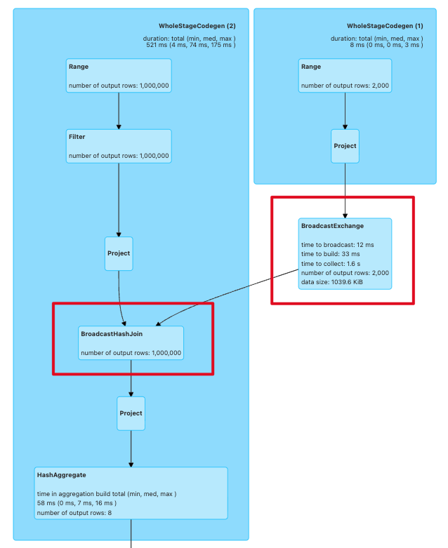
broadcast phase 的 SQL plan：dimension side 經過 BroadcastExchange，再與 fact side 進行 BroadcastHashJoin

畫面中 BroadcastExchange 顯示它建立了 2,000 rows、約 1039.6 KiB 的 broadcast relation。這個數字比單看「2,000 rows」更有意義：Spark 真正要送往每個 Executor 的是序列化後的 relation。真實 job 是否適合 broadcast，還要看欄位寬度、資料型別、每個 Executor 的 memory，以及同時有多少 broadcast datasets 存活。

Job DAG 也讓我看見資料移動的範圍。join 的 fact-side Stage 沒有在 BroadcastHashJoin 前出現依 product_id 的 Exchange；DAG 中的 Exchange 位於 join 後的 HashAggregate，它屬於最後 count() 的彙總。

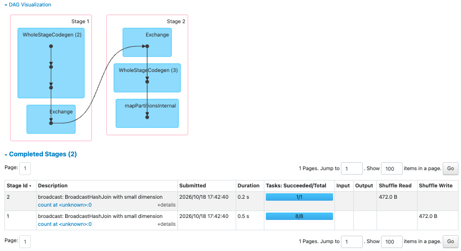
broadcast Job 的 DAG：BroadcastHashJoin 在 fact-side Stage 中完成；後方的 Exchange 來自 count() 聚合

Completed Stages 表證實這個尾端 shuffle 很小：上游 Stage 寫出 472.0 B，最後一個單 task Stage 讀回同樣的 472.0 B。這是八個 partial counts 合併成一個最終 count 的資料，而不是 1,000,000 rows 為 join 重新分配。

這個細節很容易讓我誤判。看到 Exchange 或 Shuffle Write 時，先問它在 DAG 的哪個位置、上下游 operator 是什麼；不能只因為某個 Job 有 shuffle，就直接說它用了 shuffle join。

同一個 broadcast execution，為什麼 UI 上有兩個 Jobs？

Jobs 頁實際留下三個 completed Jobs。第一個是 Spark 準備 broadcast relation 的 Job，有一個 Stage、八個 tasks；第二個才是標示為 broadcast 的 count action，有兩個 Stages、九個 tasks。第三個是接下來的 shuffle join。

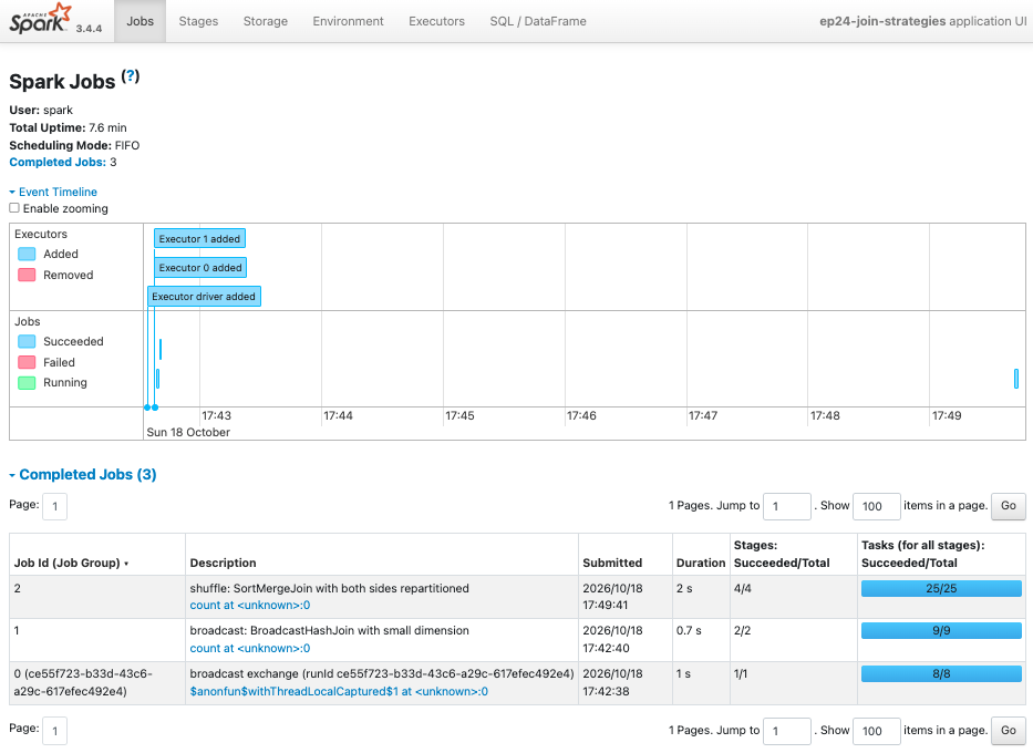
Jobs 頁顯示 broadcast exchange 的準備 Job、broadcast join Job，以及 shuffle join Job

這也延續 Ep22 的時間層級：一個 SQL execution 的完成時間，和某一個 Job 的 duration 不一定相同。broadcast relation 的建立可以形成獨立 Job；閱讀 UI 時要把 Description、Job IDs、DAG 與 SQL plan 放在一起，才不會把前置工作漏掉。

SortMergeJoin：兩側先依 join key shuffle，再排序後合併

第二個 phase 停用 auto-broadcast 後，formatted physical plan 的 dimension branch 明確出現：

Exchange hashpartitioning(product_id, 8)
    ↓
Sort(product_id)
    ↓
SortMergeJoin

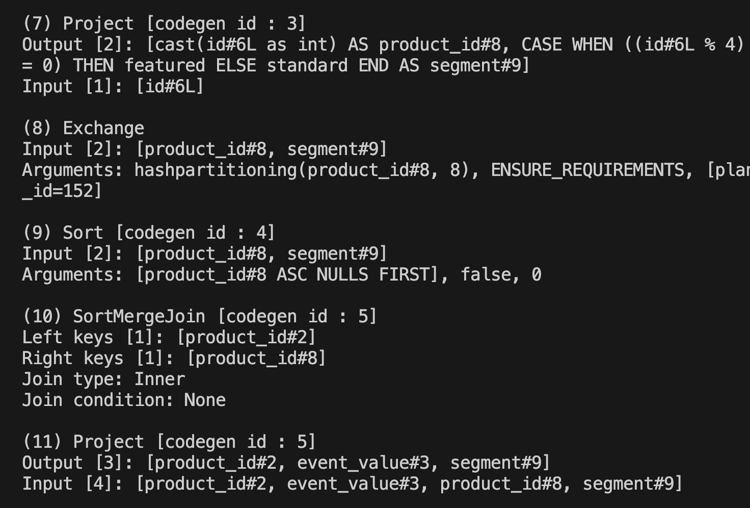
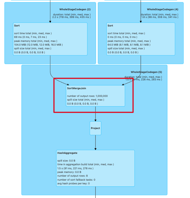
shuffle phase 的 formatted plan：dimension branch 先依 product_id hash partition，再排序並進入 SortMergeJoin

fact branch 也遵循同樣規則。因為兩側原本都沒有被保證依 product_id 分布，Spark 必須替兩邊各建立 Exchange。SQL plan 裡的兩個 Sort 收斂到同一個 SortMergeJoin，就是這個策略的骨架。

shuffle phase 的 SQL plan：兩個已排序的輸入分支匯入 SortMergeJoin

Job DAG 將這份 plan 轉成可量化的資料流。Stage 3 與 Stage 4 各有八個 tasks，分別寫出 14.6 KiB 與 972.9 KiB shuffle data；後續 Stage 5 的八個 tasks 讀回 987.5 KiB，進行 SortMergeJoin，然後才為 count() 寫出 472.0 B。

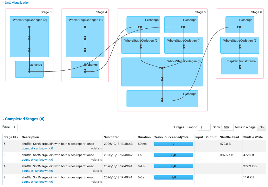
shuffle Job 的 DAG 與 Stage metrics：join 前有兩個 Exchange，Stage 5 讀回 987.5 KiB shuffle data

這是比單看 duration 更可靠的對照。這次 shuffle Job 有四個 Stages、25 個 tasks；broadcast count action 有兩個 Stages、九個 tasks。資料很小，所以 Jobs 頁分別只顯示 2 秒和 0.7 秒，不能把這些數字當成一般環境的效能比例；但 Stages、Exchange 與 Shuffle Read／Write 清楚說明兩種策略做了不同的工作。

plan 和 UI 合起來，才知道該問哪個問題

先看到的訊號	這次能確認的事	下一個要問的問題
`BroadcastHashJoin` + `BroadcastExchange`	小的一側被複製給 Executors；大型一側無須為 join key shuffle。	broadcast relation 的序列化大小、Executor memory 與同時執行的查詢是否允許？
`SortMergeJoin` + 兩側 `Exchange`	join 前兩側依 key 重分配；shuffle 是策略的一部分。	哪一側大？join key 有沒有 skew？資料能否提早 filter 或只選必要欄位？
join 後的小型 Exchange	下游 aggregation 或 count 還有自己的資料交換。	這個 Exchange 是 join 所需，還是後續 operator 所需？
少數 shuffle task 同時有巨大 records 與 duration	可能又回到 key 分布不均。	回看 Ep23：hot key 是否讓某個 partition 變成 straggler？

先由 physical plan 確認 Spark 選了哪種 join，再用 DAG 與 Stage metrics 驗證資料真的如何移動；這比直接調整 broadcast threshold 更有方向。

這次我真正學到的是什麼？

同一句 fact.join(dimension, "product_id") 背後，可以是把小表送到每個 Executor 的 BroadcastHashJoin，也可以是兩側都重新分配與排序的 SortMergeJoin。這個差異會具體出現在 BroadcastExchange、Exchange、Sort、Stage 數、task 數與 shuffle metrics。

這次我也學到，UI 出現 shuffle 不足以判定 join strategy；它可能只是 count() 或下游 aggregation 的尾端彙總。先將 Exchange 接回相鄰的 operators，再看 physical plan，才能分辨它是 join 的必要資料移動，還是下一步計算造成的交換。

下一篇會從 join 與 shuffle 回到資料讀取端：當 task 數量很多、每個 task 卻很短時，小檔案如何讓 Spark 忙著啟動與排程工作，而不是有效處理資料。