Ref.: TensorFlow exercises

昨天的文章大概講解了TensorFlow，今天來練習幾個Exercises。

Quick Introduction to pandas

之後會頻繁用到pandas這個python library，這個訓練裡主要要學會4件事情:

• 認識Dataframe, Series
• 操作Dataframe, Series
• import data from csv
• 用reindex打亂data

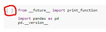
紅色圈圈可以執行，點擊code可以編輯

一開始，先引入pandas

from __future__ import print_function

import pandas as pd
pd.__version__

Dataframe是由rows跟named columns組成，而Series則是指單一一欄。也就是說，Dataframe由Series跟每個Series的名稱組成。

city_names = pd.Series(['San Francisco', 'San Jose', 'Sacramento'])
population = pd.Series([852469, 1015785, 485199]) #少一個會怎樣?

pd.DataFrame({ 'City name': city_names, 'Population': population })

這裡分別宣告了Series，然後去組成dataframe。可以試試看某個Series少一個element會怎樣。

california_housing_dataframe = pd.read_csv("https://download.mlcc.google.com/mledu-datasets/california_housing_train.csv", sep=",")
california_housing_dataframe.describe()

這邊則是把CSV吃進Dataframe，並用describe看看有興趣的統計數值。
然後要畫出某列的柱狀圖也很簡單: california_housing_dataframe.hist('housing_median_age')

接著是對Dataframe的一些操作

#我修改了某部分的code，讓大家看一些細微差異
cities = pd.DataFrame({ 'City name': city_names, 'Population': population })

# sub-dataframe
print(type(cities[['City name']]))
print(cities[['City name']])

# Series
print(type(cities['City name']))
print(cities['City name'])

See, [[]]會變成Dataframe, []則是回傳Series。

# Dataframe中'City name' series的第二個
print(type(cities['City name'][1]))
cities['City name'][1]

# Dataframe中第0列開始取2列
print(type(cities[0:2]))
cities[0:2]

接著一些對Series的運算:

import numpy as np

# 取populatioin series 的log運算
np.log(population)

# Series 每個除以1000
population / 1000.

# 每個element做個別運算(val > 1000000)
population.apply(lambda val: val > 1000000)

最有趣的，你還可以對同一個Dataframe命名一個新的column，並賦予意義:

cities['Area square miles'] = pd.Series([46.87, 176.53, 97.92])
# Populatioin density不存在在原本的Cities dataframe裡
cities['Population density'] = cities['Population'] / cities['Area square miles']
cities

Exercise 1 賦予一個新欄位，意義是"名稱是San開頭，且area > 50"
Solution 打開就看到答案囉

接著玩玩index / reindex

#都加上了print，範例中沒加是因為它code在最後執行，會印出執行結果(function定義除外)
print(city_names.index) # Series有 index
print(cityies.index)    # Dataframe 也有 index
cities.reindex(np.random.permutation(cities.index))

Exercise 2 玩看看如果reindex超出個數、或傳入的array中有element不在原本index裡會怎樣。

First Steps with TensorFlow

終於到了練習TensorFlow的part，這範例裡有

• LinearRegressor
• Predict
• Evaluate with Root Mean Squared Error
• Improve hyperparameters

不囉嗦，先引入函數

from __future__ import print_function

import math

from IPython import display
from matplotlib import cm
from matplotlib import gridspec
from matplotlib import pyplot as plt
import numpy as np
import pandas as pd
from sklearn import metrics
import tensorflow as tf
from tensorflow.python.data import Dataset

tf.logging.set_verbosity(tf.logging.ERROR)
pd.options.display.max_rows = 10
pd.options.display.float_format = '{:.1f}'.format

# import data
california_housing_dataframe = pd.read_csv("https://download.mlcc.google.com/mledu-datasets/california_housing_train.csv", sep=",")

# Prepare to run SGD
california_housing_dataframe = california_housing_dataframe.reindex(
    np.random.permutation(california_housing_dataframe.index))
# Scale median_house_value values
california_housing_dataframe["median_house_value"] /= 1000.0

好，前置作業做完(引入library、載入資料、shuffle)。接下來，定義一下我們的feature columns，有兩種類型的feature column:

1. Categorical Data: 可分類的數據資料
2. Numerical Data: 數值類型的資料
   在TensorFlow裡要先使用feature_columns construct儲存feature column的定義，如下面的tf.feature_column.numeric_column

# Define the input feature: total_rooms.
my_feature = california_housing_dataframe[["total_rooms"]] #dataframe

# Configure a numeric feature column for total_rooms.
feature_columns = [tf.feature_column.numeric_column("total_rooms")]
print(feature_columns) # output: [_NumericColumn(key='total_rooms', shape=(1,), default_value=None, dtype=tf.float32, normalizer_fn=None)]

然後呢，定義target，並定義linear_regressor:

targets = california_housing_dataframe["median_house_value"]
# Use gradient descent as the optimizer for training the model.
my_optimizer=tf.train.GradientDescentOptimizer(learning_rate=0.0000001)
my_optimizer = tf.contrib.estimator.clip_gradients_by_norm(my_optimizer, 5.0)

# Configure the linear regression model with our feature columns and optimizer.
# Set a learning rate of 0.0000001 for Gradient Descent.
linear_regressor = tf.estimator.LinearRegressor(
    feature_columns=feature_columns,
    optimizer=my_optimizer
)

用GradientDescentOptimizer train model，並用clip_gradients_by_norm確保Gradient不會太大。

可以注意到這邊有 tf.estimator 跟 tf.contrib.estimator 兩個estimator，主要差別是contrib是一些還在實驗中、隨時可能會改變的estimator。

def my_input_fn(features, targets, batch_size=1, shuffle=True, num_epochs=None):
    """Trains a linear regression model of one feature.
  
    Args:
      features: pandas DataFrame of features
      targets: pandas DataFrame of targets
      batch_size: Size of batches to be passed to the model
      shuffle: True or False. Whether to shuffle the data.
      num_epochs: Number of epochs for which data should be repeated. None = repeat indefinitely
    Returns:
      Tuple of (features, labels) for next data batch
    """
  
    # Convert pandas data into a dict of np arrays.
                                             
    # print(dict(features).items())         
    # print(dict(features).items()[0])      
    # print(dict(features).items()[0][1])     
    # print(np.array(dict(features).items()[0][1]))
    
    features = {key:np.array(value) for key,value in dict(features).items()}  
    # Construct a dataset, and configure batching/repeating.
    ds = Dataset.from_tensor_slices((features,targets)) # warning: 2GB limit
    ds = ds.batch(batch_size).repeat(num_epochs)
    
    # Shuffle the data, if specified.
    if shuffle:
      ds = ds.shuffle(buffer_size=10000)
    
    # Return the next batch of data.
    features, labels = ds.make_one_shot_iterator().get_next()
    return features, labels

中間註解了四個print，有練習的人可以複製看看這四個print印出來什麼，會更清楚for loop在幹嘛。
還有batch, repeat, shuffle 說明可以看這邊，簡單來說就是隨機打亂(shuffle)並取一定大小的資料(batch)，然後要不要受週期影響(repeat)。

之後就是給個input size去 train 一定次數(step) model，然後跑predict，接著評估MSE

_ = linear_regressor.train(
    input_fn = lambda:my_input_fn(my_feature, targets),
    steps=100
)

prediction_input_fn =lambda: my_input_fn(my_feature, targets, num_epochs=1, shuffle=False)
predictions = linear_regressor.predict(input_fn=prediction_input_fn)
predictions = np.array([item['predictions'][0] for item in predictions])

# Print Mean Squared Error and Root Mean Squared Error.
mean_squared_error = metrics.mean_squared_error(predictions, targets)
root_mean_squared_error = math.sqrt(mean_squared_error)
print("Mean Squared Error (on training data): %0.3f" % mean_squared_error)
print("Root Mean Squared Error (on training data): %0.3f" % root_mean_squared_error)

這邊引入RMSE，它能讓scale更接近target。

接著最後一個part，畫圖看成效:

sample = california_housing_dataframe.sample(n=300)
# Get the min and max total_rooms values.
x_0 = sample["total_rooms"].min()
x_1 = sample["total_rooms"].max()

# Retrieve the final weight and bias generated during training.
weight = linear_regressor.get_variable_value('linear/linear_model/total_rooms/weights')[0]
bias = linear_regressor.get_variable_value('linear/linear_model/bias_weights')

# Get the predicted median_house_values for the min and max total_rooms values.
y_0 = weight * x_0 + bias 
y_1 = weight * x_1 + bias

# Plot our regression line from (x_0, y_0) to (x_1, y_1).
plt.plot([x_0, x_1], [y_0, y_1], c='r')

# Label the graph axes.
plt.ylabel("median_house_value")
plt.xlabel("total_rooms")

# Plot a scatter plot from our data sample.
plt.scatter(sample["total_rooms"], sample["median_house_value"])

# Display graph.
plt.show()

先取300個sample畫點、決定x_min, x_max，進一步透過最佳化後的weight, bias算出y_min, y_max，然後用plot畫出線、scatter畫sample點

這部分差不多到這裡結束，因為它下面就是參數化train_model function，然後去看每個步驟train出來的linear regression，或者用不同的feature去train看看會不會比較好。

Synthetic Features and Outliers

這部分跟上面滿像的，只是要自己去定義feature，並把自己定義的feature餵進train_model，甚至更進一步透過觀察hist柱狀圖把比較奇葩的值拔掉，再餵進去train_model看看結果。建議大家實際操作看看比較有感！