今天來用scikit-learn實作一下線性迴歸
這次我們試試看boston這個資料庫（連結）
boston這個資料庫中有波士頓房價與一些因素，例如與上班區域的距離(DIS)、居民密度(ZN)等等
但是線性迴歸只需要一個變數就好，因此底下我是選DIS這個欄位來做預測

import matplotlib.pyplot as plt
import numpy as np
from sklearn import datasets, linear_model
from sklearn.model_selection import train_test_split
from sklearn.metrics import mean_squared_error

boston = datasets.load_boston()

features = boston.feature_names  #可以看看有哪些feature欄位
print(features)

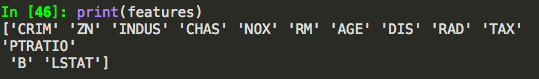
#我要第七個欄位來當feature
X =boston.data[:, np.newaxis, 7]   #the 7th feature is DIS 
y = boston.target
X_train, X_test, y_train, y_test = train_test_split(X, y, test_size=0.3)  #test_size預設是0.25

確認一下只有取一個欄位，也看一下train跟test的比例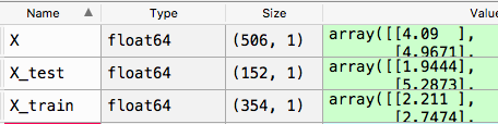

沒事的話就來弄模型吧～～～～
其實我習慣叫做y_result,但是好像有人會叫做predict_y之類的ＸＤ就自己認得就好了～

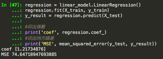
regression = linear_model.LinearRegression()
regression.fit(X_train, y_train)
y_result = regression.predict(X_test)

#印出係數
print('coef', regression.coef_)
#印出均方誤差
print('MSE', mean_squared_error(y_test, y_result))

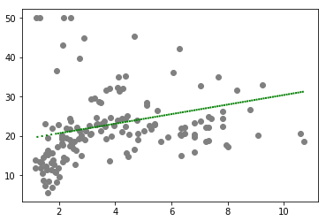
接下來來畫畫圖～

plt.scatter(X_test, y_test,  color='grey')
plt.plot(X_test, y_result, color='green', linewidth=2, linestyle=':')

plt.show()

然後這是我把每個feature丟進去測試的結果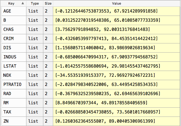

均方誤差越小越好，發現是LSTAT這個feature最有相關，官方文件解釋如下：

LSTAT % lower status of the population
QQ難過

裡面也可以看到有些feature跟房價是負相關，像是AGE, CRIM, INDUS, LSTAT, NOX等等

最後的程式碼：

import matplotlib.pyplot as plt
import numpy as np
from sklearn import datasets, linear_model
from sklearn.model_selection import train_test_split
from sklearn.metrics import mean_squared_error

boston = datasets.load_boston()

features = boston.feature_names  #可以看看有哪些feature欄位
print(features)
#我要第七個欄位來當feature

dic = {}
for i in range(0, 13):
    X =boston.data[:, np.newaxis, i]   #the 7th feature is DIS 
    y = boston.target
    
    X_train, X_test, y_train, y_test = train_test_split(X, y, test_size=0.3)  #test_size預設是0.25
    
    regression = linear_model.LinearRegression()
    regression.fit(X_train, y_train)
    y_result = regression.predict(X_test)
    
    #印出係數
    print('coef', regression.coef_)
    #印出均方誤差
    print('MSE', mean_squared_error(y_test, y_result))
    
    dic[features[i]] = [regression.coef_[0], mean_squared_error(y_test, y_result)]
    plt.scatter(X_test, y_test,  color='grey')
    plt.plot(X_test, y_result, color='green', linewidth=2, linestyle=':')
    
    plt.show()

print(dic)