前言

最近開始記錄學習Tensorflow相關的程式，這篇主要紀錄較常用的API使用方法，若想了解API的參數可前往官網。
在Tensorflow中會以張量為主做計算，張量其實就是一個描述一個R空間的說法，簡單來看能把它看為在描述常數或向量。

資料處理

Session和eval

Session在Tensorflow主要用來初始化和執行計算等等，若沒使用Session執行則不會進行計算，而也可以使用Eager API取代Session，但這邊主要紀錄Session。
而還有另一個選擇，使用eval函數結果和Session是一樣的但必須把Session打開才能使用如範例。

範例

1. 宣告一個字串常數，並使用run輸出。

words = tf.constant('Hello World !')
with tf.Session() as session:
    assert words.eval() == session.run(words)
    print(session.run(words))

隨機數

在Tensorflow當中也有與numpy類似宣告隨機數的方法，以下介紹常用的。

範例

1. 宣告隨機數值為正態分布，均值0、標準差1、大小10*10、型態float、名為matrix的矩陣(張量)。

matrix = tf.random_normal([10,10], mean=0.0,stddev=1.0, dtype=tf.float32, name="matrix")

2. 宣告隨機數值為正態分布，均值0、標準差1、大小10*10、型態float、名為matrix的矩陣(張量)並丟棄大於2個標準偏差的值重新產生隨機值。

matrix = tf.truncated_normal([10,10], mean=0.0,stddev=1.0, dtype=tf.float32, name="matrix")

3. 宣告隨機數值，範圍為最小為10、最大為100、大小10*10、型態float、名為matrix的矩陣(張量)。

matrix = tf.random_uniform ([10,10], minval=10, maxval=100, dtype=tf.float32, name="matrix")

其中還有tf.set_random_seed(value)，只要固定value則每次亂數產生結果則會一致，而還可在上述三個函數當中加入seed=value結果也會一樣。

4. 宣告0，大小10*10、型態float、名為matrix的矩陣(張量)。

matrix = tf.zeros([10,10], dtype=tf.float32, name="matrix")

5. 宣告1，大小10*10、型態float、名為matrix的矩陣(張量)。

matrix = tf.ones([10,10], minval=10, maxval=100, dtype=tf.float32, name="matrix", seed=1)

常數constant

constant在Tensorflow中代表一個常數，不可變更。

範例

1. 宣告字串常數。

words = tf.constant('Hello World !')

2. 宣告數值為0、型態float、大小3*3、名為matrix的矩陣(張量)。

matrix = tf.constant(0, dtype=tf.float32, shape=[3, 3], name="matrix")

3.1

value1 = tf.constant(2)
value2 = tf.constant(3)
print(value1)
with tf.Session() as session:
    assert value1.eval() == session.run(value1)
    print("sum = " + str(session.run(value1 + value2)))
    print("mul = " + str(session.run(value1 * value2)))

變數Variable

Variable在Tensorflow使用assign這API來改變給予它值如下圖範例。
首先initial_value為初始化常量或張量，再使用assign加入變數中，在使用value1保存，而最一開始宣告則是 value1 = tf.Variable(5, name="value1", dtype=tf.int64)。而還有較方便的API能初始化Variable，像是tf.global_variables_initializer()，使用Session執行，若要指定則加入feed_dict(後面會講到相關用法)。再來介紹它的其他用法。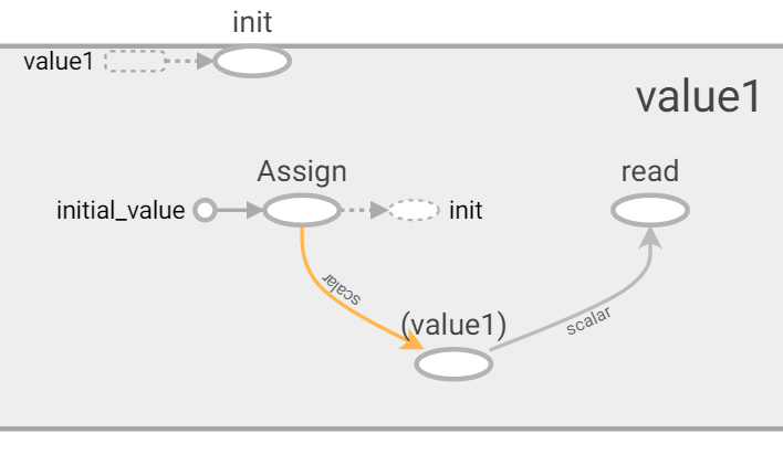

範例

1. assign將10放入變數在存入value2。

value1 = tf.Variable(5, name="value1", dtype=tf.int64)
value2 = value1.assign(10)

2. 將值改為20，必須先初始化張量。

value1 = tf.Variable(5, name="value1", dtype=tf.int64)
init_variable = tf.global_variables_initializer()
with tf.Session() as session:
    session.run(init_variable)
    value1.load(20)

3.使用tf.random_uniform初始化和np.random.rand初始化。

value1 = tf.Variable(tf.random_uniform([10,10], minval=10, maxval=100, dtype=tf.float32), name="value1")
value2 = tf.Variable(np.random.rand(10, 10), name="value2")

佔位符placeholder

在人工智慧當中，每次學習輸入的數據都不同，而placeholder可使得方便輸入不同的新數據，如下範例。

範例

1. input為一個型態float、大小N*20的placeholder， 而這裡要設計一個output為input與weights矩陣相乘加上biases位移量。
   輸入參數使用feed_dicts對應宣告的變數名稱代入即可輸出結果。這裡可以看到feed_dicts的內容可以讓我們任意更動，使得操錯彈性更佳。

# init
input = tf.placeholder(tf.float32, shape=[None, 20] ,name='input')
weights = tf.Variable(tf.random_uniform([20, 10], -1, 1), name='weights')
biases = tf.Variable(tf.zeros(10), name='biases')
output = tf.matmul(input, weights) + biases
init_var = tf.global_variables_initializer()

# output
with tf.Session() as session:
    session.run(init_var)
    feed_dicts = { input: np.random.rand(1000, 20) }
    print(session.run(output, feed_dict=feed_dicts))

get_variable

在Tensorflow當中提供了一個可以依照name直接存取Variable的函數get_variable，這樣的好處是不用一直創建新的Variable還有可以方便取得上一層所訓練的權重。
註：後面會介紹到可視化網頁，主要依照name來去呈現，若每次一直創建新的Variable呈現出來的數據就幾乎沒甚麼參考性。

範例

1.此範例使用Variable做單層感知器，執行兩次後比對能發現兩者的name和值是不同的，接著往下看使用get_variable的範例。

def layer(input, weights_shape, biases_shape):
    w = tf.Variable(tf.random_uniform(weights_shape, minval=-1, maxval=1), name="w")
    b = tf.Variable(tf.zeros(biases_shape), name="b")

    print("W Name : ", w.name)
    print("B Name : ", b.name)

    return tf.matmul(input, w) + b

# init
input1 = tf.Variable(tf.random_uniform([2, 2], -1, 1))

# process
output1 = layer(input1, [2, 2], [2])
output2 = layer(input1, [2, 2], [2])

init_value = tf.global_variables_initializer()
# output
with tf.Session() as session:
    session.run(init_value)
    print(session.run(output1))
    print(session.run(output2))

2.此範例使用get_variable做單層感知器，執行兩次後比對能發現兩者的name和值是相同的，第一次初始化會使用到initializer這相關物件或者是constent類型的Tensor，這裡呼叫了兩次則要使用tf.get_variable_scope().reuse_variables()函數設置get_variable可重複使用。相信你已經注意到get_variable_scope這函數，接著我們往下介紹。

def layer(input, weights_shape, biases_shape):
    weights = tf.random_uniform_initializer(minval=-1, maxval=1)
    biases = tf.zeros_initializer()
    w = tf.get_variable("w", weights_shape, initializer=weights)
    b = tf.get_variable("b", biases_shape, initializer=biases)

    print("W Name : ", w.name)
    print("B Name : ", b.name)

    return tf.matmul(input, w) + b

# init
input1 = tf.Variable(tf.ones([2, 2]))

# process
output1 = layer(input1, [2, 2], [2])
tf.get_variable_scope().reuse_variables()
output2 = layer(input1, [2, 2], [2])

init_value = tf.global_variables_initializer()
# output
with tf.Session() as session:
    session.run(init_value)
    print(session.run(output1))
    print(session.run(output2))

variable_scope

使用variable_scope則區域內的name都會加上variable_scope的name，假設scope名稱為scope，則原先是w會變為scope/w，而scope就能方便分開處理區域間的變數，若要在區域間重複使用name則必須設置reuse，如以下範例。

範例

1. 承get_variable，改用variable_scope，這裡介紹兩種簡單的方法。

• 方法一加入reuse=tf.AUTO_REUSE。
• 方法一加入scope.reuse_variables()。

with tf.variable_scope("scope", reuse=tf.AUTO_REUSE) as scope:
    input1 = tf.Variable(tf.random_uniform([2, 2], -1, 1))
    layer(input1, [2, 2], [2])
    #scope.reuse_variables()
    layer(input1, [2, 2], [2])

訊息

在執行時候會發現有其他的輸出資訊，我們可以設置TF_CPP_MIN_LOG_LEVEL來隱藏。

範例

1.沒設定時預設是1，設置2時只會顯示Warring和Error，設置3時只會顯示Error。

import os
os.environ['TF_CPP_MIN_LOG_LEVEL'] = '2'

concat串接陣列

範例

1.real_datas1、real_datas2、real_datas3皆是隨機數值大小[10, 2]，使用concat便可以將三者陣列合併，axis=0為列合併，也就是合併結果大小為[30, 2]，由此可知axis=1大小為[10, 6]以此類推。
``
real_datas1 = tf.random_uniform([10, 2], minval=0, maxval=5, name="real_datas1")
real_datas2 = tf.random_uniform([10, 2], minval=10, maxval=15, name="real_datas2")
real_datas3 = tf.random_uniform([10, 2], minval=20, maxval=25, name="real_datas3")

real_datas = tf.concat([real_datas1, real_datas2, real_datas3], axis=0, name="real_datas")
``

negative

範例

1.假設value=[1, 2, 3]，則result=[-1, -2, -3]。

result = tf.negative(value)

top_k

範例

1. 取出value的前K個最大值和索引位置。

(values, indices) = tf.nn.top_k(value, k)

gather

範例

1. 使用near_indexs(索引位置)取出對應的real_labels(值)。

tf.gather(real_labels, near_indexs, name="near_labels")

one_hot

範例

1. 假設near_labels為資料標籤，class_type為標籤種類數量，on_value為有值設定1，off_value無值設定0，最後即會返回near_labels的one-hot。

tf.one_hot(indices=near_labels, depth=class_type, on_value=1, off_value=0, name="one_hot_labels")

可視化資料

Graphs

當在執行Seesion流程時，想讓流程可視化，而TensorBoard則可幫助我們方便實現，只要將Seesion的
graph放入TensorBoard的函數FileWriter，它變會幫你儲存所有流程。
最後打開命令提視窗輸入tensorboard --logdir=儲存路徑，即可在預設網頁http://localhost:6006看到執行結果。

範例

1. 寫入矩陣相乘流程圖。

matrix1 = tf.Variable(tf.random_uniform([20, 20], minval=-1, maxval=1), name="matrix1")
matrix2 = tf.Variable(tf.random_uniform([20, 10], minval=-1, maxval=1), name="matrix2")
output = tf.matmul(matrix1, matrix2)
init_value = tf.global_variables_initializer()
with tf.Session() as session:
    writer = tf.summary.FileWriter("logs/", graph=session.graph)
    session.run(init_value)

結果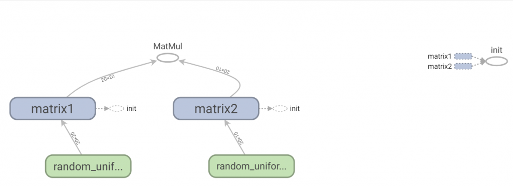

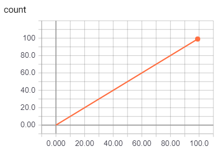
Scalar

在人工智慧當中可以使用Scalar來記錄每一次準確度、損失數值等等，最後結果類似一張折線圖。

範例

1. 使用merge_all函數取得目前設定可視化的集合，而這裡就是tf.summary.scalar("count", input)，最後跑迴圈並將運行summary_op寫入檔案，最後結果如下圖畫出0~100

input = tf.placeholder(tf.int32, name="input")
tf.summary.scalar("count", input)

summary_op = tf.summary.merge_all()

with tf.Session() as session:
    summary_writer = tf.summary.FileWriter("log/", session.graph)
    for index in range(100):
        summary_str = session.run(summary_op, feed_dict={input: index})
        summary_writer.add_summary(summary_str, index)

Histogram

TensorBoard提供了一個數據分布直方圖，讓我們參考資料的分布是否與我們預測的類似，或是資料A與資料B的差異，而資料越多所分布的資料也會相對較準確。

範例

1. 使用高斯分布製作三張不同的直方圖，分別是均值改變、標準差改變和兩者改變，如圖與我們預測的結果是類似的。(使用高斯主要是因為我們知道均值改變是大小偏移，而標準差則是控制高度，而高斯分布的圖也是我們較熟悉的)

input = tf.placeholder(tf.float32, name="input")
tf.summary.histogram("histogram1", tf.random_normal([500], mean=input))
tf.summary.histogram("histogram2", tf.random_normal([500], stddev=input))
tf.summary.histogram("histogram3", tf.random_normal([500], mean=input, stddev=input))

summary_op = tf.summary.merge_all()

with tf.Session() as session:
    summary_writer = tf.summary.FileWriter("log/", session.graph)
    for index in range(100):
        summary_str = session.run(summary_op, feed_dict={input: index})
        summary_writer.add_summary(summary_str, index)

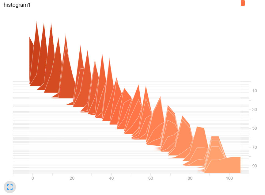
圖一，改變mean。

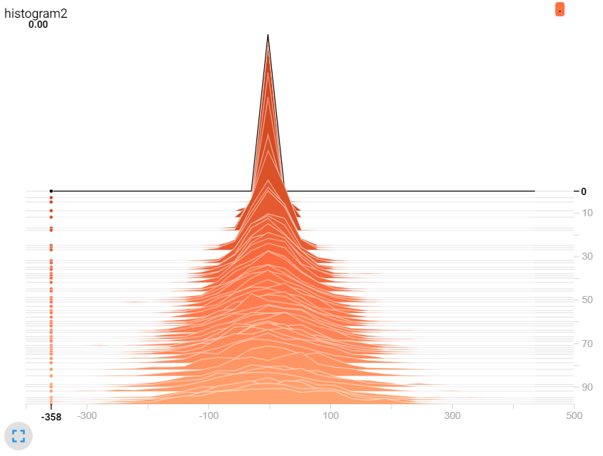
圖二，改變stddev。

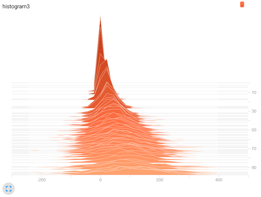
圖三，兩者改變。

結語

雖然還有很多使用方法沒介紹到，但這些作法目前可以讓我們省下更多時間撰寫程式，往後會持續更新基本使用方法。若有錯誤地方可以留言或私訊謝謝。

參考網址與書籍

[1] https://www.tensorflow.org/api_docs/python/tf
[2] https://github.com/aymericdamien/TensorFlow-Examples
[3] 籃子軒(譯者)（2018）。Deep Learning深度學習基礎｜設計下一代人工智慧演算法。台灣：歐萊禮。