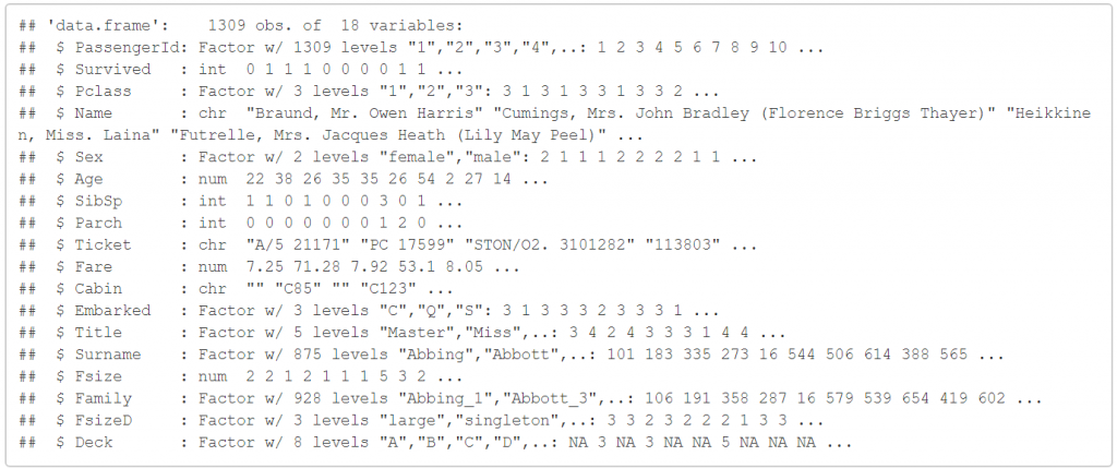
接續上次(中集)我們所做的事情，我們已經把Age的資料都給補齊了，我們來回顧一下上次最後的資料:

str(full)

現在我們想要新增一個新的變數， Child 和 Mother 。

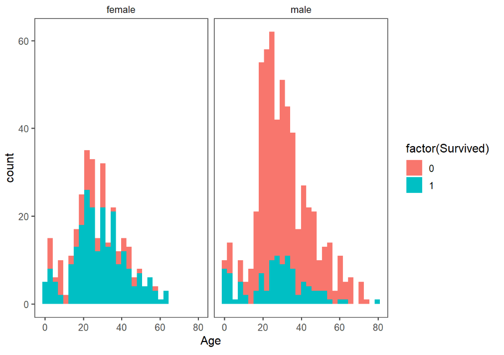
在這之前，想先來看一下性別與存活率之間的關係。

# First we'll look at the relationship between age & survival
ggplot(full[1:891,], aes(Age, fill = factor(Survived))) + 
  geom_histogram() + 
  # I include Sex since we know (a priori) it's a significant predictor
  facet_grid(.~Sex) + 
  theme_few()

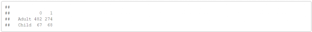
以及創建 Child 和 Mother ，我們定義所謂 Child 就是小於18歲的人，反之就是成人。

# Create the column child, and indicate whether child or adult
full$Child[full$Age < 18] <- 'Child'
full$Child[full$Age >= 18] <- 'Adult'

# Show counts
table(full$Child, full$Survived)

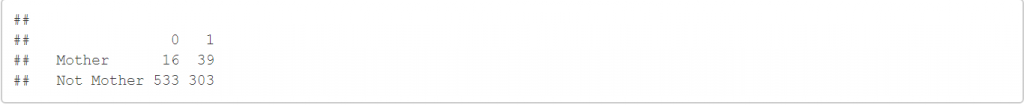
接著是 Mother ，這邊定義母親是女性，且直系親屬大於1人，且不是Miss的稱謂，並且年齡大於18歲。

# Adding Mother variable
full$Mother <- 'Not Mother'
full$Mother[full$Sex == 'female' & full$Parch > 0 & full$Age > 18 & full$Title != 'Miss'] <- 'Mother'

# Show counts
table(full$Mother, full$Survived)

把剛剛做好的新變數轉換成 factor

# Finish by factorizing our two new factor variables
full$Child  <- factor(full$Child)
full$Mother <- factor(full$Mother)

如此一來，我們所需要的變數大致都完成了，接下來我們要預測存活率！還記得我們在上集的時候，資料是分成訓練集以及測試集，現在我們把他們拆解回來。

# Split the data back into a train set and a test set
train <- full[1:891,]
test <- full[892:1309,]

並且選好一個seed，開始機器學習吧！
我們選上我們覺得較為重要的變數，先用訓練集做出我們的model:

# Set a random seed
set.seed(754)

# Build the model (note: not all possible variables are used)
rf_model <- randomForest(factor(Survived) ~ Pclass + Sex + Age + SibSp + Parch + 
                                            Fare + Embarked + Title + 
                                            FsizeD + Child + Mother,
                                            data = train)

# Show model error
plot(rf_model, ylim=c(0,0.36))
legend('topright', colnames(rf_model$err.rate), col=1:3, fill=1:3)

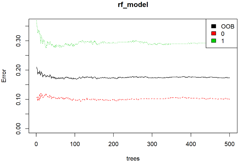
由上圖，我們黑線表示我們的錯誤率大概低於20%左右，所以算是一個還可以的模型。

接著我們可以試著看一下各個變數的重要性。

# Get importance
importance    <- importance(rf_model)
varImportance <- data.frame(Variables = row.names(importance), 
                            Importance = round(importance[ ,'MeanDecreaseGini'],2))

# Create a rank variable based on importance
rankImportance <- varImportance %>%
  mutate(Rank = paste0('#',dense_rank(desc(Importance))))

# Use ggplot2 to visualize the relative importance of variables
ggplot(rankImportance, aes(x = reorder(Variables, Importance), 
    y = Importance, fill = Importance)) +
  geom_bar(stat='identity') + 
  geom_text(aes(x = Variables, y = 0.5, label = Rank),
    hjust=0, vjust=0.55, size = 4, colour = 'red') +
  labs(x = 'Variables') +
  coord_flip() + 
  theme_few()

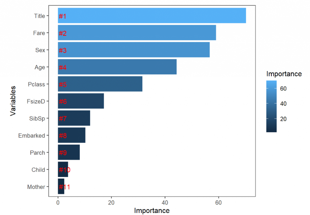
看來之前所製作的 Title 是一個蠻有用的變數，不過後來製作的其他變數就沒有那麼成功了。也有可能只是model並不是做的那麼完善，但是還是很值得可以欣賞 Megan 所做的這些嘗試。

最後我們當然要來預測我們的測試集的存活率:

# Predict using the test set
prediction <- predict(rf_model, test)

# Save the solution to a dataframe with two columns: PassengerId and Survived (prediction)
solution <- data.frame(PassengerID = test$PassengerId, Survived = prediction)

# Write the solution to file
write.csv(solution, file = 'rf_mod_Solution.csv', row.names = F)

最後我們來看一下我們預測的結果(solution)和標準答案的差異，並且算一下預測成功率。先把標準答案的資料給讀進來。

gender_submission <- read.csv('F:/Users/yueh/Desktop/titanic08/gender_submission.csv', stringsAsFactors = F)

solution$submission<-as.factor(gender_submission$Survived)
table(solution$Survived, solution$submission)

因此，我們知道預測成功率是88.9%，這次的分享就到這邊，謝謝大家。