4.1 Equal width discretisation
4.2 Equal Frequency discretisation
4.3 Discretisation using decision trees
將變數下的資料值(可以是ordinal categorical variable or numeric variable)排序並放入所屬區間(intervals, bins or buckets),這個過程也稱為分箱(binning)。
分隔變數(discretize variables)可用的方法如下:
這個方法將資料值放進N個寬度相同的區間,變數下資料的範圍和區間的數目決定區間的寬度。
寬度(width) = (最大值max value - 最小值min value) / N
雖然沒有嚴格的規定如何決定N的數目,但基本上以不超過10個為原則。還要注意一點,如果原始資料的分布是偏態(skewed)分布,這個方法不會改善資料的分布狀況。
我們可以使用pandas或scikit-learn 來對資料做分隔。
以 Kaggle 的 Titanic 資料集中的"年齡"變數來說明:
import pandas as pd
import numpy as np
import matplotlib.pyplot as plt
%matplotlib inline
import pylab
import scipy.stats as stats
from sklearn.model_selection import train_test_split
# for discretization
from sklearn.preprocessing import KBinsDiscretizer

data = pd.read_csv('../input/titanic/train.csv', usecols=['Age', 'Fare','Survived'])
data.head
Rec-no.|Survived | Age | Fare
------------- | -------------
0| 0 | 22.0 | 7.2500|
1 | 1 | 38.0| 71.2833|
2 | 1| 26.0 | 7.9250|
3| 1| 35.0 | 53.1000|
4 | 0| 35.0 | 8.0500|
.. | ... | ... | ...|
886| 0 | 27.0| 13.0000|
887| 1 | 19.0| 30.0000|
888 | 0 | NaN | 23.4500|
889| 1 | 26.0 | 30.0000|
890 | 0| 32.0 | 7.7500|
# first fill the missing data of the variable age, with a random sample of the variable

def impute_na(data, variable):
    # function to fill na with a random sample
    df = data.copy()

    # random sampling
    df[variable+'_random'] = df[variable]

    # extract the random sample to fill the na
    random_sample = df[variable].dropna().sample(df[variable].isnull().sum(), random_state=0)

    # pandas needs to have the same index in order to merge datasets
    random_sample.index = df[df[variable].isnull()].index
    df.loc[df[variable].isnull(), variable+'_random'] = random_sample

    return df[variable+'_random']

data['Age'] = impute_na(data, 'Age')
將資料分成訓練和測試集
X_train, X_test, y_train, y_test = train_test_split(data[['Age', 'Fare','Survived']],                                              data.Survived, test_size=0.3, random_state=0)
X_train.shape, X_test.shape
((623, 3), (268, 3))
(1)使用pandas
找出資料範圍並將其切成10個相同寬度的區間。
age_range = X_train['Age'].max() - X_train['Age'].min()
print(age_range)

# divide the range into 10 equal-width bins
print(age_range / 8)
79.58
9.9475
min_value = int(np.floor( X_train['Age'].min()))
max_value = int(np.ceil( X_train['Age'].max()))

# let's round the bin width
inter_width = int(np.round(age_range/10))

min_value, max_value, inter_width
(0, 80, 8)
找出每個區間的界線值
intervals = [i for i in range(min_value, max_value+inter_width, inter_width)]

intervals
[0, 8, 16, 24, 32, 40, 48, 56, 64, 72, 80]
把每筆資料的區間範圍寫入age_disc欄位。
# discretise Age
X_train['age_disc'] = pd.cut(x=X_train['Age'],
                               bins=intervals,
                               include_lowest=True)

print(X_train[['Age', 'age_disc']].head(10))
/| Age| age_disc
------------- | -------------
857| 51.0 | (48.0, 56.0]
52 | 49.0 | (48.0, 56.0]
386| 1.0 | (-0.001, 8.0]
124| 54.0| (48.0, 56.0]
578| 19.0 | (16.0, 24.0]
549| 8.0 | (-0.001, 8.0]
118| 24.0| (16.0, 24.0]
12 | 20.0 | (16.0, 24.0]
157| 30.0| (24.0, 32.0]
127| 24.0| (16.0, 24.0]
查看每個區間的資料數目
# check the number of observations per bin

X_train['age_disc'].value_counts()
| (16.0, 24.0] | 146 |
|---|---|
| (24.0, 32.0] | 145 |
| (32.0, 40.0] | 116 |
| (40.0, 48.0] | 62 |
| (-0.001, 8.0] | 52 |
| (48.0, 56.0] | 34 |
| (8.0, 16.0] | 34 |
| (56.0, 64.0] | 24 |
| (64.0, 72.0] | 8 |
| (72.0, 80.0] | 2 |
| Name: age_disc, dtype: int64 |
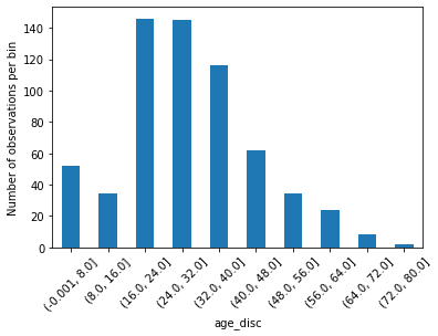
繪製每個區間資料數量的成長條圖
# plot the number of observations per bin

X_train.groupby('age_disc')['Age'].count().plot.bar()
plt.xticks(rotation=45)
plt.ylabel('Number of observations per bin')
對測試資料做區隔
# discretise the variables in the test set
X_test['age_disc'] = pd.cut(x=X_test['Age'],
                              bins=intervals,
                              include_lowest=True)
X_test.head()
比較訓練集和測試集的區間資料分布情形。
# determine proportion of observations in each bin
t1 = X_train['age_disc'].value_counts() / len(X_train)
t2 = X_test['age_disc'].value_counts() / len(X_test)

# concatenate aggregated views
tmp = pd.concat([t1, t2], axis=1)
tmp.columns = ['train', 'test']

# plot
tmp.plot.bar()
plt.xticks(rotation=45)
plt.ylabel('Number of observations per bin')

原始資料中年齡和存活的比較圖。
fig = plt.figure()
fig = X_train.groupby(['Age'])['Survived'].mean().plot()
fig.set_title('Normal relationship between Age and Survived')
fig.set_ylabel('Survived')

做分隔後的資料中年齡和存活的比較圖。
fig = plt.figure()
fig = X_train.groupby(['age_disc'])['Survived'].mean().plot(figsize=(12,6))
fig.set_title('Normal relationship between variable and target')
fig.set_ylabel('Survived')

(2)使用scikit-learn
disc = KBinsDiscretizer(n_bins=10, encode='ordinal', strategy='uniform')
disc.fit(X_train[['Age']])
KBinsDiscretizer(encode='ordinal', n_bins=10, strategy='uniform')
各區間的界線值儲存在disc.bin_edges 中
disc.bin_edges_
array([array([ 0.42 , 8.378, 16.336, 24.294, 32.252, 40.21 , 48.168, 56.126,
64.084, 72.042, 80. ])], dtype=object)
train_t = disc.transform(X_train[['Age']])
train_t = pd.DataFrame(train_t, columns = ['Age'])
test_t = disc.transform(X_test[['Age']])
test_t = pd.DataFrame(test_t, columns = ['Age'])
train_t.head()
| / | Age |
|---|---|
| 0 | |
| 1 | 6.0 |
| 2 | 0.0 |
| 3 | 6.0 |
| 4 | 2.0 |
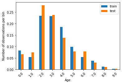
比較訓練集和測試集的區間資料分布情形。
t1 = train_t.groupby(['Age'])['Age'].count() / len(train_t)
t2 = test_t.groupby(['Age'])['Age'].count() / len(test_t)

tmp = pd.concat([t1, t2], axis=1)
tmp.columns = ['train', 'test']
tmp.plot.bar()
plt.xticks(rotation=45)
plt.ylabel('Number of observations per bin')