近年來深度學習使用在許多比賽中,但幾乎都使用ensemble(集成)的方式或是使用龐大的模型,這有個很嚴重的問題,那就是成本過高無法落地(除了原本就很昂貴的設備),因此近幾年也有許多人設計適用於嵌入式裝置的模型,而Neural Architecture Search(NAS)便是解決辦法之一,它能自動搜尋模型架構找到較為適合的架構,並且在效能上也能夠有一定的表現,甚至有些NAS在訓練時也能限制FPS和模型大小等等,如此一來在嵌入式裝置也能夠輕易地使用並且獲得好的效能。
此篇文章要介紹的是Sequential Greedy Architecture Search(SGAS)[1],SGAS是基於gradient descent(梯度下降演算法,GD)來找架構,這裡我使用Convolutional neural network(CNN)作為範例 ,除了GS以外還有evolutionary algorithm (演化是演算法, EA)和reinforcement learning(強化學習,RL)等等方式能夠找架構。想了解更多可參考AutoML Survey[2]。
首先簡單的先了解SGAS的貢獻。
註:假設Cell和Block是相同的東西
在開始進入SGAS時要先知道什麼是Cell(Block),因為SGAS是在找出一個可能較好的Cell(Block)。這裡使用Resnet[3]為例,我們常常會聽到ResNet18/34/50/101/151...,而後面數字是代表經過了N層的運算層,其中運算層如卷積層和池化層等等,而Cell其實就是將幾個運算層組合起來,如下圖一(a)為ResNet-38的Cell,由此可知道ResNet-38是使用許多個Cell(a)所堆疊起來的網路,同理可知圖一(b)也是一樣,除此之外不同的Cell也會得到不同的效能。因此有許多人設計了不同的Cell來提升效能,而這篇論文是使用可微分與可加性來去找出最佳的Cell,如此一來能夠因應不同的資料集並且減少人工設計的成本。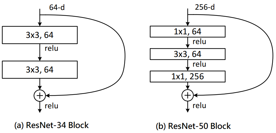
圖一,來源[3]。
從ResNet上面可以看到每一個箭頭代表著一種運算層,而在SGAS中則是先定義N種運算層(3x3卷積層、最大池化層、5x5卷積層...),也就是說第N層到第N+1層從原先只計算一個運算層變為需要計算N個運算層,如圖二(a),不同顏色的箭頭代表著不同的運算層,而N個運算層會乘上一個對應的權重(訓練出來的)做相加。
接著會先經過訓練後,在N個運算層中選出一個較為重要的運算層,其餘的則忽略,而這就是剪枝,如圖二(b),經過Greedy Decision在第0個節點和第1個節點選出藍色線,再來經過訓練後相同的經過Greedy Decision選擇要剪枝的節點,如圖二(c),反覆此步驟直到每個節點都剪枝完畢,如圖二(d)。
簡單的例子:假設輸入(1, 3, 32, 32)大小的資料。
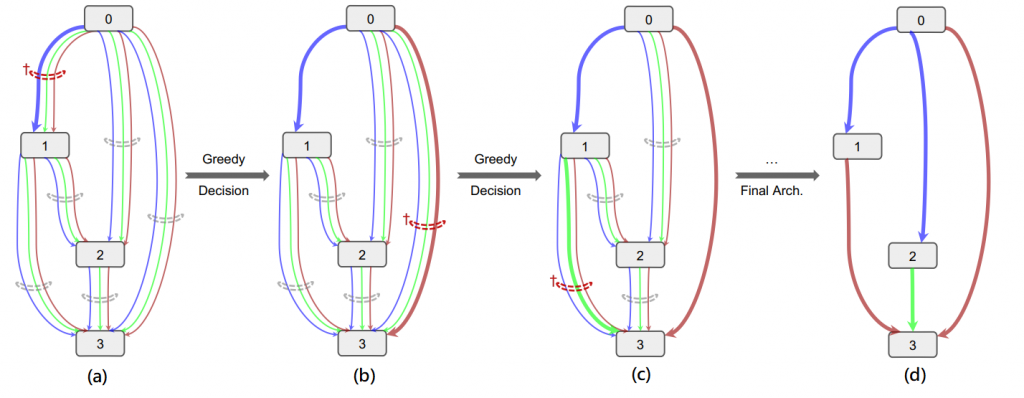
圖二,來源[2]。
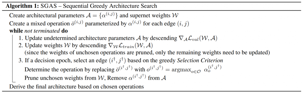
這裡直接附上SGAS演算法,如圖三,其中i和j代表著不同的節點,alpha代表運算層的重要度(權重),W代表整體網路的權重,這裡與上述的流程是相同的,只是用演算法的形式寫出。
SGAS主要使用了三個公式作為Greedy Decision的選擇標準。
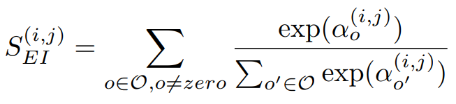
公式一,來源[2]。
Selection Certainty
第二個公式為計算alpha(i, j)的確定性,其中i、j為不同的節點。公式二則延續公式一,只是多使用entropy來計算平均的確定性。詳細公式如公式二。
這裡舉個簡易的例子來看出entropy的特性,其中entropy公式為x*log(x),可以看到越接近1或0的entropy都會比較大,因此能夠利用entropy的特性來計算出不確定性(越接近0確定性越大)。而要計算確定性只要加上1即可。
1.機率為0.9的entropy為0.9 * log(0.9) = -0.04,反之確定性=0.96。
2.機率為0.1的entropy為0.1 * log(0.1) = -0.1,反之確定性=0.9。
3.機率為0.5的entropy為0.5 * log(0.1) = -0.15,反之確定性=0.85。
上述的例子可以得知0.5的不確定性較大,可以反應出未收斂或模型產生矛盾等等情況。
註:計算一次極端狀況能知道Selection Certainty是補足Edge Importance的不足。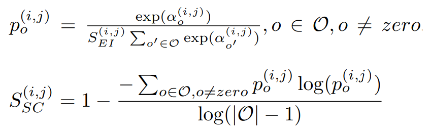
公式二,來源[2]。
Selection Stability
第二個公式為計算alpha(i, j)的穩定性,其中i、j為不同的節點。若只考慮公式一和公式二,可以知道兩者僅僅只考慮當下的alpha(i, j),這有可能會產生不穩定情形,例如第一次決策時的機率是0.1,第二次決策時的機率是0.9,第三次0.1,第四次0.9,這時就會有不穩定的情況,因此SGAS考慮了T個歷史紀錄,用來計算彼此的交集,這樣能夠將穩定度也考慮進去。詳細公式如公式三。
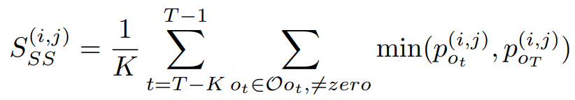
公式三,來源[2]。
SGAS使用了上述三個公式做評估,假設都是獨立機率則相乘即可獲得分數,而分數又分為Cri.1公式四和Cri.2公式五,差別在於有無考慮歷史訊息(Selection Stability)。
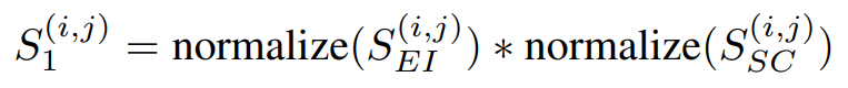
公式四,來源[2]。
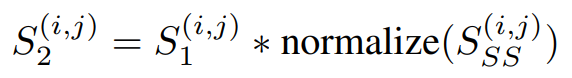
公式五,來源[2]。
GitHub位置:/sgas/cnn/model_search.py
一般的網路運算層基本上只有一個運算層,如3x3卷積層、5x5卷積層、3x3空洞卷積層....,而SGAS運算層定義為包含八種運算層,如下。
PRIMITIVES = [
    'none',
    'max_pool_3x3',
    'avg_pool_3x3',
    'skip_connect',
    'sep_conv_3x3',
    'sep_conv_5x5',
    'dil_conv_3x3',
    'dil_conv_5x5'
]
MixedOp:當無選擇的索引(未被剪枝)則計算八種運算層乘上權重的合,若有選擇的索引(已剪枝)則選擇該層運算做為輸出。
class MixedOp(nn.Module):
    def forward(self, x, weights, selected_idx=None):
        if selected_idx is None:
            return sum(w * op(x) for w, op in zip(weights, self._ops))
        else:  # unchosen operations are pruned
            return self._ops[selected_idx](x)
Cell:SGAS用兩個Node做為輸入,分別是前一個Cell的輸出(s0),現在Cell的輸出(s1),這種想法其實有點類似ResNet和DenseNet,甚至未來可以嘗試使用CSPNet的想法來減少計算量,而這裡的**_steps表示操作次數,可以當作是Cell深度的上限(預設4),每計算一次就可以得到更高階的特徵,並且會將輸出加入states list內以供下次操作使用,這裡其實也隱含著類似ResNet和DenseNet**的想法,因為下一層還能夠使用上一層的輸入進行運算,可以讓網路自行決定要使用低階特徵或是高階特徵。
註:這裡特別的地方是states list的數量隨著增加,但輸出的數量是不變的,因為會將所有states list經過MixedOp的輸出進行相加,這想法也就是特徵融合。
class Cell(nn.Module):
    def forward(self, s0, s1, weights, selected_idxs=None):
        s0 = self.preprocess0(s0)
        s1 = self.preprocess1(s1)

        states = [s0, s1]
        offset = 0
        for i in range(self._steps):
            o_list = []
            for j, h in enumerate(states):
                if selected_idxs[offset + j] == -1: # undecided mix edges
                    o = self._ops[offset + j](h, weights[offset + j])
                    o_list.append(o)
                elif selected_idxs[offset + j] == PRIMITIVES.index('none'): # pruned edges
                    continue
                else: # decided discrete edges
                    o = self._ops[offset + j](h, None, selected_idxs[offset + j])
                    o_list.append(o)
            s = sum(o_list)
            offset += len(states)
            states.append(s)

        return torch.cat(states[-self._multiplier:], dim=1)
Network _initialize_alphas:初始化每一個Cell內的運算層權重,與上述Cell迴圈相同,而產生亂數的大小是運算層種類大小(8種運算),而這裡較為特別的地方是,分為alphas_normal和alphas_reduce權重,alphas_normal代表無需下採樣的Cell,而alphas_reduce代表需要下採樣的Cell,(部份研究)會分為兩個區塊的原因可能是下採樣通常會設定不同的stride或池化層等等,因此這操作與無須下採樣的Cell是稍微不同的,所以會分為兩個區塊進行。
Network forward:會先計算alphas權重,再呼叫Cell進行計算,與一般網路差別在於權重。
Network check_edges:在剪枝完後呼叫,會限制每一次操作(深度),若以有max_num_edges個已決策的節點則其餘節點可以忽略。這個函數在限制計算複雜度,而當限制越寬鬆(max_num_edges越大)則運算量越大與訓練時間越久。
class Network(nn.Module):
    def _initialize_alphas(self):
        k = sum(1 for i in range(self._steps) for n in range(2 + i))
        num_ops = len(PRIMITIVES)

        self.alphas_normal = []
        self.alphas_reduce = []
        for i in range(self._steps):
            for n in range(2 + i):
                self.alphas_normal.append(Variable(1e-3 * torch.randn(num_ops).cuda(), requires_grad=True))
                self.alphas_reduce.append(Variable(1e-3 * torch.randn(num_ops).cuda(), requires_grad=True))
        self._arch_parameters = [
            self.alphas_normal,
            self.alphas_reduce,
        ]

    def forward(self, input):
        s0 = s1 = self.stem(input)
        for i, cell in enumerate(self.cells):
            if cell.reduction:
                selected_idxs = self.reduce_selected_idxs
                alphas = self.alphas_reduce
            else:
                selected_idxs = self.normal_selected_idxs
                alphas = self.alphas_normal

            weights = []
            n = 2
            start = 0
            for _ in range(self._steps):
                end = start + n
                for j in range(start, end):
                    weights.append(F.softmax(alphas[j], dim=-1))
                start = end
                n += 1

            s0, s1 = s1, cell(s0, s1, weights, selected_idxs)

        out = self.global_pooling(s1)
        logits = self.classifier(out.view(out.size(0), -1))
        return logits

    def check_edges(self, flags, selected_idxs, reduction=False):
        n = 2
        max_num_edges = 2
        start = 0
        for i in range(self._steps):
            end = start + n
            num_selected_edges = torch.sum(1 - flags[start:end].int())
            if num_selected_edges >= max_num_edges:
                for j in range(start, end):
                    if flags[j]:
                        flags[j] = False
                        selected_idxs[j] = PRIMITIVES.index('none') # pruned edges
                        if reduction:
                            self.alphas_reduce[j].requires_grad = False
                        else:
                            self.alphas_normal[j].requires_grad = False
                    else:
                        pass
            start = end
            n += 1

        return flags, selected_idxs
GitHub位置:/sgas/cnn/architect.py
Architect有使用到unrolled來控制是否要添加train data的hessian矩陣(梯度的方向)到優化器內,而這並不是該論文重點(預設false,其它dataset訓練也無使用),因此就先略過,有興趣可找相關文獻觀看。
使用validation data更新未剪枝的的alphas權重。(神經網路無更新)
class Architect(object):
  def _backward_step(self, input_valid, target_valid):
    loss = self.model._loss(input_valid, target_valid)
    loss.backward()
GitHub位置:/sgas/cnn/train_search.py
現在知道主要的Network架構也知道驗證更新參數時使用的是Architect,接著就是greedy decision的算法,這裡就按照上述所講的演算法和公式一步一步的講解。
訓練所對應的演算法就是1.使用validation data來更新alpha和2.使用train data來更新weights。
參數:
train_queue:train dataloader(Pytorch Class)
valid_queue:validation dataloader(Pytorch Class)
model:train model
architect:class of update alpha
input:train data
target:train target
input_search:validation data
target_search:validation target
def train(train_queue, valid_queue, model, architect, criterion, optimizer, lr, epoch):
    ...

        # Algorithm 1. Update undetermined architecture parameters(only alpha)
        architect.step(input, target, input_search, target_search, lr, optimizer, unrolled=args.unrolled)

        # Algorithm 2. Update weights W
        optimizer.zero_grad()
        logits = model(input)
        loss = criterion(logits, target)

    ...
註解對應到上述的公式1~5。演算法對應到3.剪枝,特別的是剪枝完還會使用model.check_edges檢查已剪枝數量,以用來決定該層是否還需要剪枝(限制剪枝和運算量)。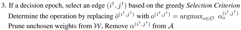
參數:
args.use_history:用來決定要不要使用歷史資料。
args.warmup_dec_epoch:能當做預訓練(不做剪枝)。
args.decision_freq:剪枝頻率。
candidate_flags:節點是否剪枝的標記。
score:將評估的標準經過正規化[0,1]相乘。
selected_edge_idx:取得最大分數的索引(貪婪算法)。
selected_op_idx:取得selected_edge_idx運算層機率最大的索引(貪婪算法),因為前面忽略non-zero層所以這裡index要+1轉回原本運算層的index。
def edge_decision(type, alphas, selected_idxs, candidate_flags, probs_history, epoch, model, args):
    mat = F.softmax(torch.stack(alphas, dim=0), dim=-1).detach()

    # Formula 1
    importance = torch.sum(mat[:, 1:], dim=-1)

    # Formula 2
    probs = mat[:, 1:] / importance[:, None]
    entropy = cate.Categorical(probs=probs).entropy() / math.log(probs.size()[1])


    if args.use_history: # SGAS Cri.2
        # Formula 3
        histogram_inter = histogram_average(probs_history, probs)
        probs_history.append(probs)
        if (len(probs_history) > args.history_size):
            probs_history.pop(0)

        # Formula 5
        score = utils.normalize(importance) * utils.normalize(
            1 - entropy) * utils.normalize(histogram_inter)

    else: # SGAS Cri.1
        # Formula 4
        score = utils.normalize(importance) * utils.normalize(1 - entropy)


    if torch.sum(candidate_flags.int()) > 0 and \
            epoch >= args.warmup_dec_epoch and \
            (epoch - args.warmup_dec_epoch) % args.decision_freq == 0:
        masked_score = torch.min(score,(2 * candidate_flags.float() - 1) * np.inf)
        selected_edge_idx = torch.argmax(masked_score)
        selected_op_idx = torch.argmax(probs[selected_edge_idx]) + 1 # add 1 since none op
        selected_idxs[selected_edge_idx] = selected_op_idx

        candidate_flags[selected_edge_idx] = False
        alphas[selected_edge_idx].requires_grad = False
        if type == 'normal':
            reduction = False
        elif type == 'reduce':
            reduction = True
        else:
            raise Exception('Unknown Cell Type')
        candidate_flags, selected_idxs = model.check_edges(candidate_flags,selected_idxs,reduction=reduction)
        print(type + "_candidate_flags {}".format(candidate_flags))
        score_image(type, score, epoch)
        return True, selected_idxs, candidate_flags

    else:
        print(type + "_candidate_flags {}".format(candidate_flags))
        score_image(type, score, epoch)
        return False, selected_idxs, candidate_flags
SGAS在NAS當中訓練速度是相當快的,而這次只運行CNN,資料集使用Cifar-10和MNIST,但一般我們遇到的資料可能不是CNN,而SGAS也考慮的了這點,因此還能用於GCN等等上(其實滿多都能用在不同地方),另外如果有時間會在打上一篇來講解如何用在Kaggle的鐵達尼號或房價預測,並且使用sklearn-AutoML來進行比較,感覺上AutoML在節省人力與實用性算是相當高的,希望未來有機會能夠在工作場所發揮。
有任何問題或筆誤歡迎留言
修改後原始碼:jupyter notebook code
修改後原始碼:Github
論文原始碼:SGAS Github
[1] Li, G., Qian, G., Delgadillo, I.C., M¨uller, M., Thabet, A., Ghanem, B.: Sgas: Sequential greedy architecture search. In: Proceedings of the IEEE Conference on
Computer Vision and Pattern Recognition (2020).
[2] X. He, K. Zhao, and X. Chu, “Automl: A survey of the state-of-the-art,” arXiv preprint arXiv:1908.00709 (2019).
[3] K. He, X. Zhang, S. Ren, and J. Sun. Deep residual learning for image recognition. In CVPR, 2016.
 Kevin
Kevin

 iThome鐵人賽