Chap.I 理論基礎

Part 1：線性代數

1. Getting Started with Equations

1-1. eval()，算數

x=6
y=10
eval('100 * x +300 +y +9')

>>  919

1-2. exec()，把 () 中的語法視作 python 語法，接著執行

exec('''
for i in range(5):
    print (f"iter time: {i}" )
''')
>>  iter time: 0
    iter time: 1
    iter time: 2
    iter time: 3
    iter time: 4

1-3. Symbol Python（sympy）

A. 解方程式 (預設右側為0)

from sympy.solvers import solve
from sympy import Symbol
x = Symbol('x')

print(solve(x**2 - 1, x))

>>  [-1, 1]

B 產生上標 (jupyter 有效 QQ)

from sympy.solvers import solve
from sympy import Symbol
x = Symbol('x')

x**4+2*x**2+3

C. 直接解方程式

from sympy.core import sympify
x, y = sympify('x, y')

print(solve([x + y + 2, 3*x + 2*y], dict=True))

>>  [{x: 4, y: -6}]

2. Linear Equations 線性方程式

2-1. Intercept (截距)

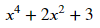
# 求 20 個 x 點對應的 y 值
import pandas as pd
import matplotlib.pyplot as plt

df = pd.DataFrame ({'x': range(-10, 11)})
df['y'] = (3*df['x'] - 4) / 2

# 作圖
plt.plot(df.x, df.y, color="0.5")
plt.xlabel('x')
plt.ylabel('y')
plt.grid()
plt.axhline()
plt.axvline()

x_i = [(1.33, 0), (0, 0)]
y_i = [[0, 0], [0, -2]]
plt.annotate('x-intercept',(1.333, 0))
plt.annotate('y-intercept',(0,-2))
plt.plot(x_i[0], x_i[1], color="r")
plt.plot(y_i[0], y_i[1], color="y
plt.show()

")

2-2. slope

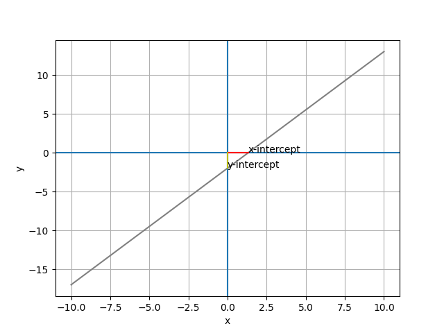
# 作圖
plt.plot(df.x, df.y, color="0.5")
plt.xlabel('x')
plt.ylabel('y')
plt.grid()
plt.axhline()
plt.axvline()

# the slope
slope = 1.5
x_slope = [0, 1]
y_slope = [-2, -2 + slope]
plt.plot(x_slope, y_slope, color='red', lw=5)
plt.savefig('pic 03.png')
plt.show()

2-3. Regression

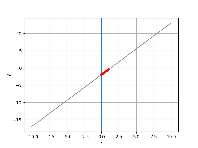
# 世界人口預測
year=[1950, 1951, 1952, 1953, 1954, ...2100]
pop=[2.53, 2.57, 2.62, 2.67, 2.71, ...10.85]

# 1. Numpy regression
x1 = np.linspace(1950, 2101, 2000)
fit = np.polyfit(year, pop, 1)
y1 = np.poly1d(fit)(x1)

# 作圖
plt.figure(num=None, figsize=(18, 10), dpi=80, facecolor='w', edgecolor='k')
plt.plot(year, pop, 'b-o', x1, y1, 'r--')
plt.show()

# 2. LinearRegression
X = np.array(year).reshape(len(year), 1)
y = np.array(pop)
from sklearn.linear_model import LinearRegression as LR
clf = LR()
clf.fit(X, y)    # 線性迴歸
print(f'y = {clf.coef_[0]:.2f} * x + {clf.intercept_:.2f}')
>> y = 0.06 * x + -116.36

# 作圖
plt.figure(num=None, figsize=(18, 10), dpi=80, facecolor='w', edgecolor='k')
x1 = np.arange(1950, 2101)
y1 = clf.coef_[0] * x1 - clf.intercept_
plt.plot(year, pop, 'b-o', x1, y1, 'r--')
plt.show()

2-4. 用 make_regression 產生亂數資料

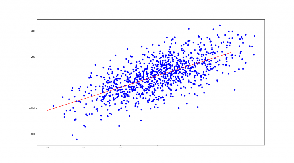
from sklearn.datasets import make_regression as mr
# n_features= : 幾個 x
# noise= : 雜訊量
# bias= : 截距
X, y= mr(n_samples=1000, n_features=1, noise=10, bias=50)

# use sklearn LinearRegression
from sklearn.linear_model import LinearRegression as LR
clf = LR()
clf.fit(X, y)
coe = clf.coef_[0]
ic = clf.intercept_
print(f' y = {coe:.2f} * x + {ic:.2f}') # 1 + {clf.coef_[1]:.2f} * x2
>> y = 89.69 * x + 52.88

# 作圖
import matplotlib.pyplot as plt
plt.figure(num=None, figsize=(18, 10), dpi=80, facecolor='w', edgecolor='k')
plt.scatter(X, y, c='b')         # 畫出 X, y 點點
X1 = np.linspace(-3, 2, 100)
plt.plot(X1, coe*X1 + ic, 'r')   # 畫出迴歸紅線
plt.show()

3. Systems of Equations 聯立方程式

Numpy 線性代數解聯立方程式
EX1. 4x - 5y = -13
-2x + 3y = 9

import numpy as np
a = np.array([[4, -5], [-2, 3]])
b = np.array([-13, 9])

print(np.linalg.solve(a, b))

>>  [3. 5.]

EX2. x + 2y = 5
y - 3z = 5
3x - z = 4

a = np.array([[1, 2, 0], [0, 1, -3], [3, 0, -1]])
b = np.array([5, 5, 4])

print(np.linalg.inv(a) @ b)

>>  [ 1.  2. -1.]

4. Exponentials, Radicals, and Logs 指數、根號和對數

4-1. Basic

import math
# 16 是 4 的幾次方
print(math.log(16, 4))

>>  2.0

# 100 是 log10 的幾次方
print(math.log10(100))

>>  2.0

# e & pi
print(math.e, math.pi) # 等同於 np.e, np.pi

>>  2.718281828459045 3.141592653589793

# 100 是 e 的幾次方
print(math.log(100, math.e))

>>  4.605170185988092

4-2. Solving Equations with Exponentials

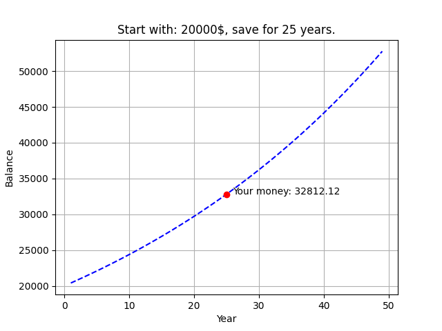
複利計算

import pandas as pd

m = int(input('請輸入你想存多少 (錢): '))
i = int(input('請輸入你想存多久 (年): '))
total_monety = m*(1.02**i)
df = pd.DataFrame ({'Year': range(1, 50)})
df['Balance'] = m*(1.02**df['Year'])

from matplotlib import pyplot as plt
plt.plot(df.Year, df.Balance, 'b--', i, total_monety, 'ro')
plt.xlabel('Year')
plt.ylabel('Balance')
plt.grid()
plt.title(f'Start with: {m}$, save for {i} years.')
plt.annotate(f'Your money: {total_monety:.2f}',(i+1, total_monety))
plt.show()

5. Polynomials 多項式

1. Adding Polynomials
2. Subtracting Polynomials
3. Multiplying Polynomials
4. Dividing Polynomials

6. Factorization 因式分解

Greatest Common Factor (最大公因數)

a = int(input('數字1: '))
b = int(input('數字2: '))
def GCD(x, y):
    while True:
        if y == 0:
            print(x)
            break
        else:
            return GCD(y, x%y)
GCD(a, b)

7. Quadratic Equations 二次方程式

7-1. Parabola 拋物線

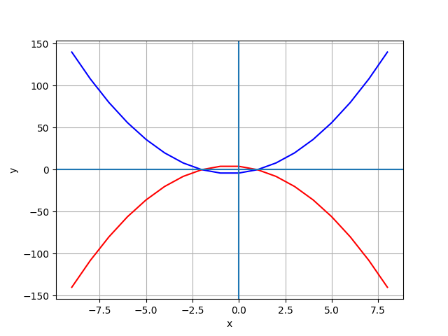
import pandas as pd
import numpy as np
from matplotlib import pyplot as plt

df = pd.DataFrame ({'x': range(-9, 9)})
df['y1'] = 2*df['x']**2 + 2 *df['x'] - 4
df['y2'] = -(2*df['x']**2 + 2*df['x'] - 4)

# 作圖
from matplotlib import pyplot as plt
plt.plot(df.x, df.y1, 'b', df.x, df.y2, 'r')
plt.plot()
plt.xlabel('x')
plt.ylabel('y')
plt.grid()
plt.axhline()
plt.axvline()
plt.show()

7-2. Parabola Vertex and Line of Symmetry 拋物線頂點與對稱線

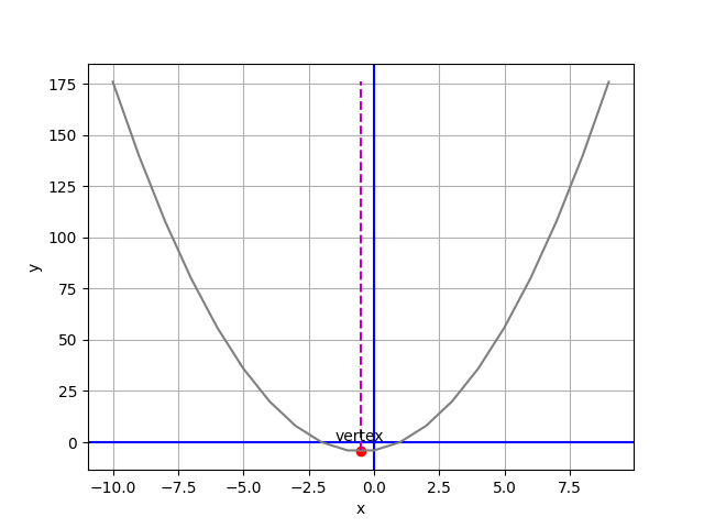
import pandas as pd
import numpy as np
import matplotlib.pyplot as plt

def plot_parabola(a, b, c):     # 代入 (2, 2, -4)
    vx = (-1*b)/(2*a)           # 極值點斜率必為0，f(x)'=2ax+b=0，x=(-b/2a)
    vy = a*vx**2 + b*vx + c     # 代入 f(x) 求極值 y 座標

    df = pd.DataFrame ({'x': np.linspace(-10, 10, 100)})
    df['y'] = a*df['x']**2 + b*df['x'] + c     # 把 x, y 輸入進 df

    # 作圖
    plt.xlabel('x')     # x 軸名稱
    plt.ylabel('y')     # y 軸名稱
    plt.grid()          # 灰色格線
    plt.axhline(c='b')  # 水平基準線
    plt.axvline(c='b')  # 垂直基準線
    xp = [vx, vx]
    yp = [df.y.min(), df.y.max()]
    plt.plot(df.x, df.y, '0.5', xp, yp, 'm--')  # 劃出拋物線 / y 最小垂直線
    plt.scatter(vx, vy, c='r')                  # 劃出 y 最小點
    plt.annotate('vertex', (vx, vy), xytext=(vx - 1, (vy + 5)* np.sign(a)))
    plt.savefig('pic 10.png')
    plt.show()

plot_parabola(2, 2, -4)

8. Function 函數

8-1. Basic

import numpy as np
import matplotlib.pyplot as plt

def f(x):
    return x**2 + 2

8-2. Bounds of a Function

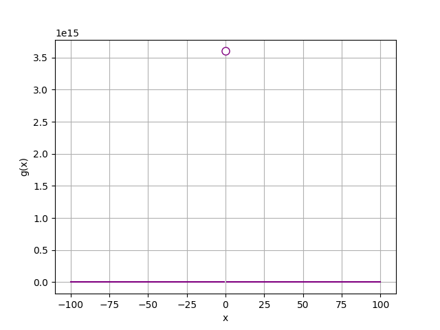
import numpy as np
import matplotlib.pyplot as plt

def g(x):
    if x != 0:
        return (12/(2*x))**2
x = range(-100, 101)
y = [g(a) for a in x]

# 作圖
plt.xlabel('x')
plt.ylabel('g(x)')
plt.grid()
plt.plot(x,y, color='purple')
plt.plot(0, g(0.0000001), c='purple', marker='o', markerfacecolor='w', markersize=8)
plt.show()

.
.
.
.
.

Homework Ans：

1. 紅酒分類：

import pandas as pd
import numpy as np
from sklearn import datasets

ds = datasets.load_wine()

X =pd.DataFrame(ds.data, columns=ds.feature_names)
y = ds.target

from sklearn.model_selection import train_test_split as tts
X_train, X_test, y_train, y_test = tts(X, y, test_size=0.1)

A. 使用 KNN 驗算法：

from sklearn.neighbors import KNeighborsClassifier as KNN

clf = KNN(n_neighbors=3)
clf.fit(X_train, y_train)
clf.score(X_test, y_test)

>> 0.78

B. 使用 LogisticRegression 驗算法：

from sklearn.linear_model import LogisticRegression as lr
clf2 = lr(solver='liblinear')
clf2.fit(X_train, y_train)
clf2.score(X_test, y_test)

>>  1.0

以上兩種模型比較後，選擇第二種模型。

此步驟是在做機器學習第八步：Evaluate Module

2. 糖尿病迴歸：

import pandas as pd
import numpy as np
from sklearn import datasets

ds = datasets.load_diabetes()

# 注意此處 X 的數值經過 standardization，固有出現年齡負值的情況。
# (X-m)/sigma，平均為 0 / 標準差為 1
X = pd.DataFrame(ds.data, columns=ds.feature_names)
y = ds.target

from sklearn.model_selection import train_test_split as tts
X_train, X_test, y_train, y_test = tts(X, y, test_size=0.2)

from sklearn.linear_model import LinearRegression
clf = LinearRegression()
clf.fit(X_train, y_train)
clf.score(X_test, y_test)

>>  0.46

額外補充：求 MSE & Coefficients

from sklearn.metrics import mean_squared_error, r2_score
y_pred = clf.predict(X_test)

# Coefficients (一次項式係數)
# y = w1*x1 + w2*x2 + w3*x3 ... w10*x10 + b
print('Coefficients: ', clf.coef_)

>>  Coefficients:  [ -42.4665896  -278.41905956  519.81553297  346.25936576 -836.62271952
      494.18394438  135.91708785  164.44984594  795.02484868   69.8608995 ]

print('Intercept: ', clf.intercept_)

>>  Intercept:  152.2877890433722

# MSE (均方誤差)：1/n * sum(y_pred-y_test)
print(f'MSE: {mean_squared_error(y_test, y_pred)}')

>>  MSE: 3161.582266519054

# Coefficient of determination (判定係數)：越接近 1 越好
print(f'Coefficient of determination: {r2_score(y_test, y_pred)}')

>>  Coefficient of determination: 0.4556662437750665

3. 小費迴歸：

import pandas as pd
import numpy as np
from sklearn import datasets

df = pd.read_csv('tips.csv')
print(df.head())

X = df.drop('tip', axis=1)   # 把'tip'丟棄
y = df['tip']                # y 為要分析的資料

# 顯示 'sex' 欄位不同的項目
print(X['sex'].unique())

>>  ['Female' 'Male']

此時若直接跑演算法，會發現評分過低，推斷為 X['day']轉化為數字時編碼問題。

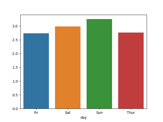
解決方式如下：

gb = df.groupby(['day'])['tip'].mean()
print(gb)
>>  Fri    2.73
    Sat    2.99
    Sun    3.26
    Thur   2.77

import seaborn as sns
import matplotlib.pyplot as plt
sns.barplot(gb.index, gb.values)
plt.show()

# 把所有值換成數字才能分析
X['sex'].replace({'Female' : 0, 'Male' : 1}, inplace=True)
X['smoker'].replace({'Yes' : 0, 'No' : 1}, inplace=True)
X['day'].replace({'Thur' : 0, 'Fri' : 0, 'Sat' : 2, 'Sun' : 3}, inplace=True)
X['time'].replace({'Lunch' : 0, 'Dinner' : 1}, inplace=True)

from sklearn.model_selection import train_test_split as tts

X_train, X_test, y_train, y_test = tts(X, y, test_size = 0.2)

from sklearn.linear_model import LinearRegression
clf = LinearRegression()
clf.fit(X_train, y_train)

clf.score(X_test, y_test)

>>  0.4