主成分分析（Principal Component Analysis, PCA），在機器學習與統計學領域中仍被廣泛應用。其主要目的就是用來分析資料、降低資料維度以及去關聯，是一種線性降維方法。在機器學習中為什麼需要降維呢？特徵（feature）不是愈多愈好嗎？其實不然，降維的優點是減少計算的時間、成本、避免維度詛咒（在樣本數沒有增加的情形下，模型的預測能力在到達一定的程度後，隨著維度的增加而減弱），也能使數據結果更容易理解，比如說將高維度的資料降到 2-3 個，方便製成 2D 或 3D圖。

整體而言，可以將 PCA 的特徵及目的整理如下：

• 將資料投影到不同維度上，以找出資料中重要的成分。

• 找出最能代表數據的主成分，並以此為基準，重新描述數據的成分表徵。

• 用以分析資料、降低維度以及去關聯性的線性降維方法 (正交變換)

  • 去關聯 (Decorrelation)：去除特徵之間的關聯性，以獨立解釋數據的特質。

  • 正交變換：保持圖形形狀和大小的轉換。

• PCA 原理：

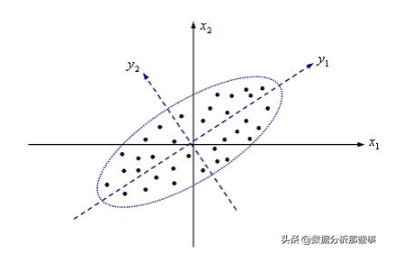
以下圖為例，許多資料點分佈於圖中。若單純以 x1 及 x2 二個向量來代表這些點，則會損失許多原始數據的訊息。此時，若將整個座標軸進行旋轉，就會產生新的座標軸 y1 及 y2。而經由旋轉而產生 y1 投影範圍的資料點有較大的離散性，即 y1 可以代表原始數據的絕大部分信息。原本需要 x1 和 x2 兩個指標才能描述的資訊，透過此方法就能以一個指標 y1 來表示就是所謂的降維。

圖片資料來源(https://kknews.cc/zh-tw/news/k6o2mgq.html)

說了這麼多降維的好處，我們就來用 Python 簡單實作一下吧！

Python PCA 實作

dataset:

乳癌數據集是一個真實的多元數據，由兩個類別組成：惡性和良性。惡性類有212個樣本，而良性類有357個樣本，其中包含跨所有類共享的 30 個特徵：半徑、紋理、周長、面積、平滑度、分形維數等，並標記病人是否患有乳癌。

首先，一次把需要的套件都引入。

from sklearn.datasets import load_breast_cancer # 引入 dataset
import numpy as np
import pandas as pd
from sklearn.preprocessing import StandardScaler # for nomalization
from sklearn.decomposition import PCA
import matplotlib.pyplot as plt # 畫圖用
%matplotlib inline

load breast dataset 時會給你 label 和 data。要取得 data 的話要用.data，要標籤則是 .target。

# get data
breast = load_breast_cancer()
breast_data = breast.data
breast_data.shape

執行結果為：
(569, 30)

# get label
breast_labels = breast.target
breast_labels.shape

執行結果為：
(569,)

接下來，把 label 和 data 組合起來，變成 dataframe

labels = np.reshape(breast_labels,(569,1))
final_breast_data = np.concatenate([breast_data,labels],axis=1)
breast_dataset = pd.DataFrame(final_breast_data)
features = breast.feature_names
features_labels = np.append(features,'label')
breast_dataset.columns = features_labels
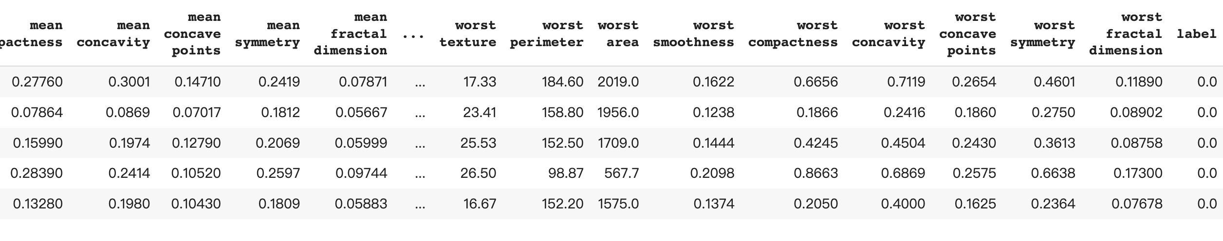
breast_dataset.head()

執行結果為：

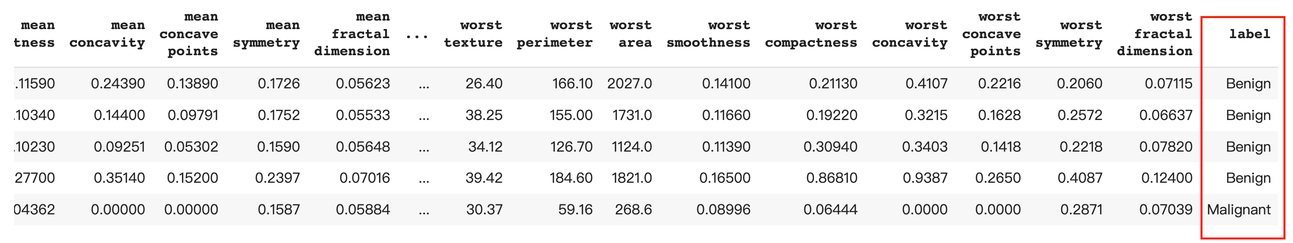
因為 dataset 中的 label 是 0 和 1 ，我們這邊換成良性 Begin (begin tumor) 和 惡性 Malignant (malignant tumor)

breast_dataset['label'].replace(0, 'Benign',inplace=True)
breast_dataset['label'].replace(1, 'Malignant',inplace=True)

執行結果為：

x = breast_dataset.loc[:, features].values
x = StandardScaler().fit_transform(x) # normalizing the features

np.mean(x),np.std(x) # check mean (0) and standard deviation (1)

執行結果為：
(-6.826538293184326e-17, 1.0) mean 接近 0 標準差為 1

feat_cols = ['feature'+str(i) for i in range(x.shape[1])]
normalised_breast = pd.DataFrame(x,columns=feat_cols)
normalised_breast.tail() # 看一下 normalized 後的結果

這裡是關鍵，把 30 維 (features) 乳癌數據使用 sklearn 導入的 PCA 投影成 2 維。

pca_breast = PCA(n_components=2) # 這邊可以自己調要幾維
principalComponents_breast = pca_breast.fit_transform(x)
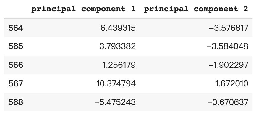
principal_breast_Df = pd.DataFrame(data = principalComponents_breast
             , columns = ['principal component 1', 'principal component 2']) 
             # 畫出 dataframe 看看

最後畫個圖看看 PCA 結果吧！

import matplotlib.pyplot as plt
%matplotlib inline


plt.figure()
plt.figure(figsize=(10,10))
plt.xticks(fontsize=12)
plt.yticks(fontsize=14)
plt.xlabel('Principal Component - 1',fontsize=20)
plt.ylabel('Principal Component - 2',fontsize=20)
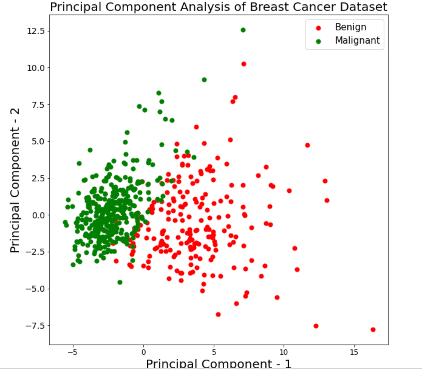
plt.title("Principal Component Analysis of Breast Cancer Dataset",fontsize=20)
targets = ['Benign', 'Malignant']
colors = ['r', 'g']
for target, color in zip(targets,colors):
    indicesToKeep = breast_dataset['label'] == target
    plt.scatter(principal_breast_Df.loc[indicesToKeep, 'principal component 1']
               , principal_breast_Df.loc[indicesToKeep, 'principal component 2'], c = color, s = 50)

plt.legend(targets,prop={'size': 15})