今天我們要實做 Feed Forward Network

前饋式神經網路是一種人工神經網路結構，也稱為前饋網路或前向傳播網路。

它是一種最基本的神經網路結構，通常由多個神經元層組成，信息傳遞方向是單向的，從輸入層經過中間隱藏層，最終到達輸出層。

在這種結構中，每一層的神經元與下一層的神經元之間建立權重連接，用於權重的調整和信息的傳遞。

Implementation

Import Library

import numpy as np
import matplotlib.pyplot as plt
import pandas as pd
import tqdm

首先我們先導入所需要的函式庫

Load data

train_x, train_y = np.load('/kaggle/input/custom-fnn/train_x.npy'), np.load('/kaggle/input/custom-fnn/train_y.npy')
test_x, test_y = np.load('/kaggle/input/custom-fnn/test_x.npy'), np.load('/kaggle/input/custom-fnn/test_y.npy')

checkpoint = np.load('/kaggle/input/custom-fnn/weights.npy', allow_pickle=True).item()
init_weights = checkpoint['w']
init_biases = checkpoint['b']

接著，我們讀取資料集 train_x.npy、train_y.npy、test_x.npy、test_y.npy

npy 檔是 numpy 專用的二進制文件，用於儲存數據

之後讀取初始網路權重 weight.npy

FNN from scracth

# number of layers: 3
# number of neurons in each layer (in order): 2048, 512, 5
# activation function for each layer (in order): relu, relu, softmax
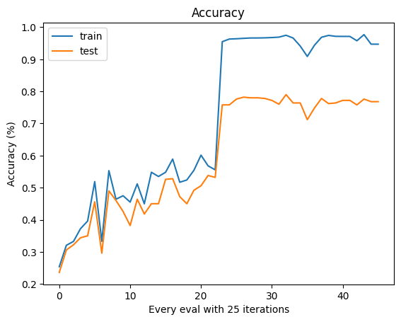
# number of training epochs: 30
# learning rate: 0.01
# batch size: 200

cache = {}

params = {
        "w1": init_weights[0], # shape: (784, 2048)
        "b1": init_biases[0], # shape: (2048, 1)
        "w2": init_weights[1], # shape: (2048, 512)
        "b2": init_biases[1], # shape: (512, 1)
        "w3": init_weights[2], # shape: (512, 5)
        "b3": init_biases[2] # shape: (5, 1)
}       

# define the activation function
def relu(x):
    return np.maximum(0, x)

def softmax(x):
    exps = np.exp(x - np.max(x, axis=1, keepdims=True))
    return exps / np.sum(exps, axis=1, keepdims=True)

def drelu(x):
    return np.where(x > 0, 1, 0)

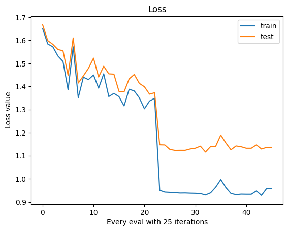
def cross_entropy_loss(y_hat, y_true):
    """
    y_hat: predicted label, shape: (batch_size, 5)
    y_true: true label, shape: (batch_size, 5)

    cross_entropy_loss = -1/m * np.sum(y_true * np.log(y_hat))
    """
    y_true = np.eye(5)[y_true]
    y_hat = softmax(y_hat)
    return -1/y_true.shape[0] * np.sum(y_true * np.log(y_hat + 1e-8))

def accuracy(y_hat, y_true):
    y_hat = np.argmax(y_hat, axis=1)
    return np.sum(y_hat == y_true) / len(y_true)

def forward(x):
    """
    x: input data, shape: (784, batch_size)
    z = x @ w + b
    a = relu(z)
    """
    cache['x'] = x
    cache['z1'] = cache['x'] @ params['w1'] + params['b1'] # (200, 784) @ (784, 2048) + (2048, 1) = (200, 2048)
    cache['a1'] = relu(cache['z1']) # (200, 2048)
    cache['z2'] = cache['a1'] @ params['w2'] + params['b2'] # (200, 2048) @ (2048, 512) + (512, 1) = (200, 512)
    cache['a2'] = relu(cache['z2']) # (200, 512)
    cache['z3'] = cache['a2'] @ params['w3'] + params['b3'] # (200, 512) @ (512, 5) + (5, 1) = (200, 5)
    cache['a3'] = softmax(cache['z3']) # (200, 5)
    return cache['a3']

def back_propagate(y, y_hat):
    """
    y: true label, shape: (batch_size, 5)
    y_hat: predicted label, shape: (batch_size, 5)
    dz = (1./m) * (y_hat - y)
    dw = a.T @ dz
    """
    y = np.eye(5)[y]
    dz3 = (1./y.shape[0]) * (y_hat - y) # (200, 5)
    dw3 = cache['a2'].T @ dz3 # (512, 200) @ (200, 5) = (512, 5)
    db3 = np.sum(dz3, axis=0).T # (5, 1)
    dz2 = dz3 @ params['w3'].T * drelu(cache['z2']) # (200, 5) @ (5, 512) * (200, 512) = (200, 512)
    dw2 = cache['a1'].T @ dz2 # (2048, 200) @ (200, 512) = (2048, 512)
    db2 = np.sum(dz2, axis=0).T # (512, 1)
    dz1 = dz2 @ params['w2'].T * drelu(cache['z1']) # (200, 512) @ (512, 2048) * (200, 2048) = (200, 2048)
    dw1 = cache['x'].T @ dz1 # (784, 200) @ (200, 2048) = (784, 2048)
    db1 = np.sum(dz1, axis=0).T # (2048, 1)
    
    grads = {
        "w1": dw1,
        "b1": db1,
        "w2": dw2,
        "b2": db2,
        "w3": dw3,
        "b3": db3,
    }
    return grads

首先，定義神經網路的模型，這模型會用於分類問題：

• 神經網路有3層：第一層有2048個神經元，第二層有512個神經元，第三層有5個神經元。
• 每一層的激活函數依次為：relu、relu、softmax。
• 訓練的時候會執行30個訓練週期（epochs）。
• 學習率為0.01，表示在每次更新模型權重時的步長大小。
• 每個訓練批次的大小為200，表示每次訓練模型時使用的樣本數量。

接下來是模型的參數（權重和偏差）的初始化，這些參數將在訓練過程中逐漸調整以適應訓練數據。

程式碼中定義了幾個函數：

• relu(x)：計算 ReLU（修正線性單元）激活函數。
• softmax(x)：計算 softmax 激活函數，用於將模型的輸出轉換為類別概率分佈。
• drelu(x)：計算 ReLU 激活函數的導數。
• cross_entropy_loss(y_hat, y_true)：計算交叉熵損失，用於評估模型的性能。
• accuracy(y_hat, y_true)：計算模型的準確率。

接下來是模型的前向傳播和反向傳播函數的定義：

• forward(x)：計算從輸入數據到模型輸出的前向傳播過程，包括線性計算和激活函數的應用。
• back_propagate(y, y_hat)：計算反向傳播過程，用於計算梯度並更新模型的權重和偏差。

反向傳播過程，我們使用 mini-batch SGD (stochastic gradient descent) 來更新參數

Result

詳細 Notebook 可以參考 Kaggle Notebook

明天要進入真實實戰部份

我們會透過 Kaggle Dataset Natural Language Processing with Disaster Tweets 來演練