EDA (進階版)

🤔 摘要寫得和原文越像，老師給的分數會越高嗎？

直覺上來說，摘要和原文一點都不像，應該會超低分，代表根本沒有在根據原文寫作；但如果和原文一字不差，應該也會很低分，因為這樣就不叫摘要了呀！叫做「把原文複製一遍」。

感覺應該是相似度要大於一個水準，但也不能完全一樣，才能拿高分吧！

❓❓但問題是，究竟什麼叫做「相似度」呢❓❓

”我喜歡你“ 和 ”吾心悦汝“ 這兩句話都是在表達相同的意思，但沒有任何一個字或詞是一樣的。
我們要怎麼寫程式判斷文本和文本之間的相似度呢？

相似度可以從 linguistic（語言學）的角度計算，也就是關注文本的表層文本結構和語言成分，而非深層語義內容。它側重於如何通過直接分析文本中的語言元素（如單詞、短語、句子結構）來評估文本之間的相似性；或者我們也可從計算Semantic(語義)相似度的角度出發，通過計算句子向量之間的相似度來評估文本的語義相似性。舉例說明如下：

• 場景設定
  假設我們有兩段文本需要比較：

  文本A："The weather is cold and rainy today."
  文本B："It's a rainy and chilly day."

  • 基於向量的語義相似度計算
    這種方法會首先將每個文本轉換為一個向量。假設我們使用了一種詞嵌入技術（如Word2Vec），每個詞都被映射到一個高維空間中的點。

    • 向量表示：每個文本轉化為詞向量的集合，然後通過某種方式（如平均、TF-IDF加權等）合成一個文本級別的向量。
    • 相似度計算：計算兩個文本向量之間的余弦相似度。
    • 結果：這種方法主要關注詞義的相似性和整體的語義內容，因此，盡管“cold”和“chilly”在字面上不同，但由於在語義上接近，兩個文本在語義上會被評為相似。

  • 基於語言學的文本相似度計算（使用ROUGE-L）
    ROUGE-L關注的是文本的表層結構，特別是詞的順序和出現頻率。

    • 分析方式：計算兩個文本之間最長公共子序列（LCS），這里是“rainy”和“day”，忽略了其他不匹配的詞。
    • 召回和精確度：評估這一LCS相對於每個文本長度的覆蓋率。
      • 結果：ROUGE-L將重點放在表面的文字匹配上，可能會低估“cold”和“chilly”的語義近似性，因為它側重於直接的文字匹配和順序。

  • 總結差異

    • 基於向量的方法 更適合於理解和比較文本的深層意義，忽略具體的表述方式，適用於內容推薦、信息檢索等需要語義理解的場景。
    • 基於語言學的方法（如ROUGE-L）則更關注文本的表層表達和結構，適用於需要評估文本保真度的場景，如文本摘要和機器翻譯質量評估。

💡 從 Linguistic 的角度計算相似度

我們首先使用 RougeL 這個指標來計算每筆資料的原文和摘要的相似度。
RougeL的計算步驟如下：

1. 最長公共子序列（LCS）：ROUGE-L度量兩個文本序列中的最長公共子序列的長度，這種方法考慮了詞序的影響並保留了文本的句法結構。
2. 召回率和精確度：通過比較LCS長度和參考文本（如人工總結）長度來計算召回率，以及LCS長度和候選文本（如自動生成總結）長度來計算精確度。
3. F-分數：結合召回率和精確度計算，提供了一個平衡兩者的評估分數。

接下來我們上代碼：

• 定義計算 rougeL 的 function

rouge = Rouge()
def get_rouge_l_score(row):
    scores = rouge.get_scores(row['text'], row['prompt_text'])
    return scores[0]['rouge-l']['f']  # f-measure of ROUGE-L

• 在 dataframe(merged)新增一個 'rouge_l_score'的column，來存放每一筆資料的 text 與 prompt_text 計算出的 rougeL分數:

merged['rouge_l_score'] = merged.progress_apply(get_rouge_l_score, axis=1)

這邊架上 progress_apply 來可視化現在計算的進度，需在文件開頭使用 tqdm 如下：

from tqdm import tqdm
tqdm.pandas()

• 計算 correlation scroe 並可視化 rougeL 和 content score 的散佈圖分佈：

correlation = merged['rouge_l_score'].corr(merged['wording'])
print(f"Correlation coefficient between ROUGE-L scores and content scores: {correlation}")

plt.figure(figsize=(10, 6))
sns.scatterplot(data=merged, x='rouge_l_score', y='wording')
sns.regplot(data=merged, x='rouge_l_score', y='wording', scatter=False, order=2, color='red')  # 二次拟合曲线
plt.title(f'Correlation coefficient between ROUGE-L scores and wording scores: {correlation:.2f}')
plt.xlabel('ROUGE-L Score')
plt.ylabel('wording Score')
plt.grid(True)
plt.show()

要計算和 wording score 的關係只需要把上面的 'content' 換成 'wording' 即可。
🔎 Findings: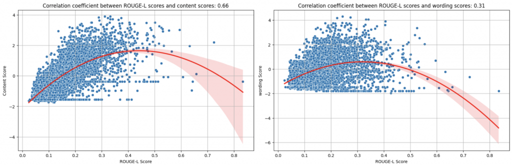

ROUGE-L的分數和 content score 的相關係數有到 0.66 分，但和 wording 卻只有 0.31 分。

從圖上可以看出，ROUGE-L Score 和 Content Score 相關性應該不是線性的，隨著 ROUGE-L的分數逐漸提高到 0.3, 0.4 左右， content score 的分數也會來到最高點，但當 ROUGE-L的分數再繼續增加，也就是摘要和原文的最長子公共字串越長，content score 就有開始下降的趨勢。

這也比較符合我們當初的預期，當摘要和原文內容、用字遣詞都差不多的時候，就失去摘要的意義了，因此在 content score 上會被懲罰。

threshold_low = 0.2
threshold_high = 0.8

# 分段統計
low_segment = merged[merged['rouge_l_score'] < threshold_low]['content'].mean()
middle_segment = merged[(merged['rouge_l_score'] >= threshold_low) & (merged['rouge_l_score'] <= threshold_high)]['content'].mean()
high_segment = merged[merged['rouge_l_score'] > threshold_high]['content'].mean()

print(f"Average Content Score for Low ROUGE-L (<{threshold_low}): {low_segment}")
print(f"Average Content Score for Middle ROUGE-L ({threshold_low}-{threshold_high}): {middle_segment}")
print(f"Average Content Score for High ROUGE-L (>{threshold_high}): {high_segment}")

Average Content Score for Low ROUGE-L (<0.2): -0.32626235284415195
Average Content Score for Middle ROUGE-L (0.2-0.8): 1.0276844195811574
Average Content Score for High ROUGE-L (>0.8): -0.382272237741744

我們如果分段去檢驗的話，摘要和原文計算出的 ROUGE-L 小於 0.2 分和大於 0.8 分的 data，他的平均 content score 都大概是 -0.3 分左右偏低；但是 ROUGE-L 屆在 0.2~0.8 分區間的 data，得到的就是比較高的平均 content score: 1.027。

💡 從 Semantic 的角度計算相似度

首先，我們先利用語言模型將 prompt_text與text轉成向量，之後再計算兩個向量的 cosine similarity，以此當作這兩個文本的相似度。

• 這邊我們選擇使用 intfloat/multilingual-e5-large 這個模型：

from transformers import AutoTokenizer, AutoModel
import torch
tokenizer = AutoTokenizer.from_pretrained('intfloat/multilingual-e5-large')
model = AutoModel.from_pretrained('intfloat/multilingual-e5-large')
device = torch.device('cuda' if torch.cuda.is_available() else 'cpu')
model.to(device)

• 定義將文本轉成向量的 function

def get_embedding(text):
    # 对文本进行分词
    encoded_input = tokenizer(text, return_tensors='pt', truncation=True, max_length=512).to(device)
    # 获取模型的输出
    with torch.no_grad():
        output = model(**encoded_input)
    # 我们取最后一层的输出的第一个token（[CLS] token）作为整个输入句子的嵌入表示
    return output.last_hidden_state[0][0]

• 定義計算向量之間的 cosine similarity 的 function

def calculate_semantic_similarity(row):
    text1 = row['text']
    text2 = row['prompt_text']
    # 获取文本嵌入
    embedding1 = get_embedding(text1)
    embedding2 = get_embedding(text2)
    # 计算余弦相似度
    return 1 - cosine(embedding1.cpu().numpy(), embedding2.cpu().numpy())

• 開始計算

merged['embedding_similarity'] = merged.progress_apply(calculate_semantic_similarity, axis=1)

🔎 Findings:

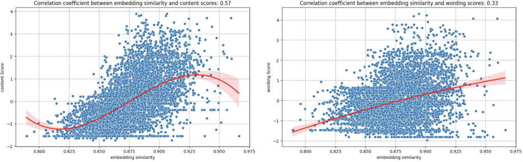
從語義角度計算的 cosine similarity score 和 content 的 correlation 只有 0.57，看起來也是有 similarity 越高分 content 分數越高的趨勢，然後相似度高於 0.925 分，content score 就會下降。

不過這個趨勢好像沒有前面用 ROUGE-L 看明顯。

這也合理，因為語義計算比較模糊，高分摘要的語意相似度也會是高分的；但是 ROUGE-L 太高分代表用字、標點符號都和原文差不多，這就很明顯是抄襲，有比較明顯的界線。

討論到這邊，我們應該可以初步下一個小節：
計算原文與摘要的相似度應該會是一個不錯的、可以拿來預測 content scrore 和 wording score 的 feature！
如果要直接用 deberta 爆 train 的話，應該也要同時放入 prompt_text 與 text 這兩個資訊。

🤔 把 content score rotate 30 度？

有神奇的網友1發現，如果我們把 content 和 wording 的 score 各為 x, y 軸畫成散佈圖，會長下面這個樣子？

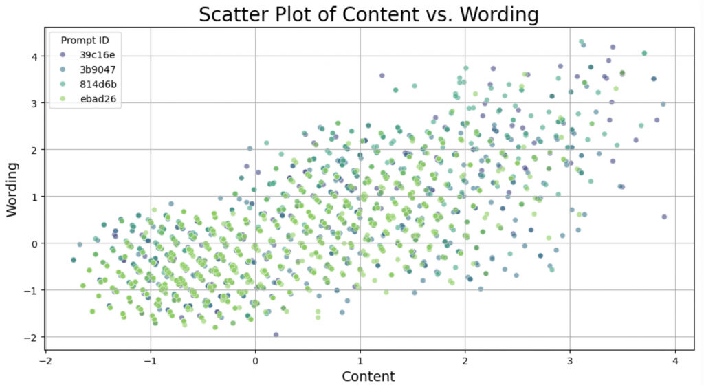
但是如果把 content 旋轉 30 度呢？

angle_deg = 30
angle_rad = np.radians(angle_deg)
rotation_matrix = np.array([[np.cos(angle_rad), -np.sin(angle_rad)],
                            [np.sin(angle_rad), np.cos(angle_rad)]])
oof_df[['content', 'wording']] = oof_df[['content', 'wording']].values.dot(rotation_matrix)

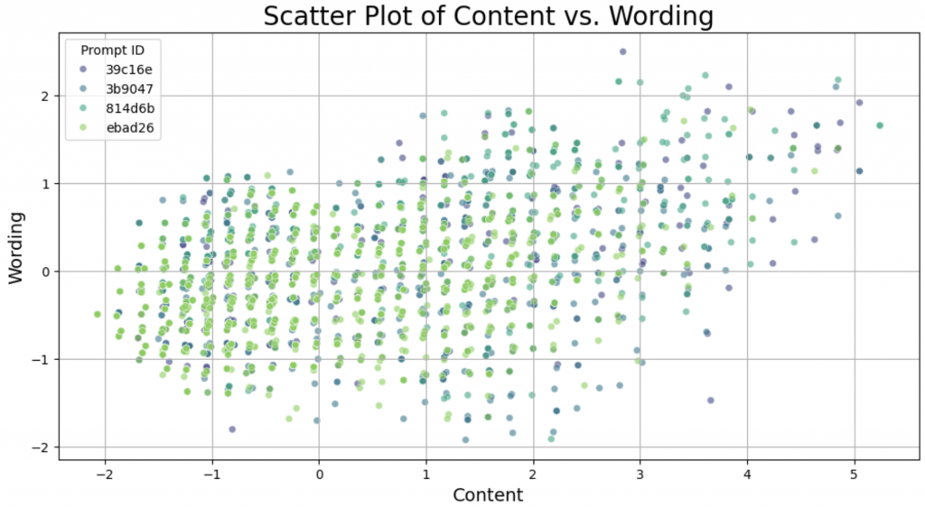
你發現了嗎？好像 content 和 wording 突然對齊了，直直地排列成一豎一豎的。並且從 content 的方向來看，可以分成 37 豎，或是我們可以說分成 37 個 cluster。

這個現象還滿有趣的，網友提出各式各樣可能的解釋，例如這可能對應到美國的等級制A+, A, A−, B+, B, B−, C+, C, C−, D+, D, D− and F.
但要怎麼利用這個現象？

🤔 為什麼會重複出現超低分的 (content, wording) pair?

但是當我們深挖 (content, wording) score 的時候，會發現整個 training set 重複出現 426 次完全相同的 (content, wording) score pair，而且分數極低：

Most common score pair: (-1.54716321678788, -1.46124482282529), Count: 426

我們把其中幾組資料的摘要print出來看看：

1. 'Tragedy much b complex, Tragedy much b complex, t must be a man that is NOT perfect, and their downfall is a result of a mistake or weakness.'
2. 'In the second paragraph Aritole explained, "A perfect tradegy, as we have seen, be arranged not on the simple but on the complex plan. It should, moreover, imitate actions which exile pity and fear, this being the distinctive mark of tragic imitation."'
3. 'Three elements of an ideal tradgedy would be very complex and "excite pity and fear", it should go from good to bad, ending in dramatic way that is the suffices "true tragic pleasure", and focus on a man who is hit with extreme difficulties.'
4. 'For nothing can be more alien to the spirit of Tragedy; it possesses no single tragic quality; it neither satisfies the moral sense nor calls forth pity or fear.'
5. 'Cause pity and fear in the audience, a person not evil or good to fall because of a mistake, and there should never be a downfall of the villain shown.'
6. "The three elements of an ideal tragedy are a plot that isn't in favor of the main character, likeable characters, and the ability to envoke fear. "

為什麼會有大量重複的超低分 (content, wording) pair 呢？

你會怎麼解釋？

我想，可能會有以下幾種猜測：

1. 這些摘要都太短了？
   但是真的是這樣嗎？平均摘要字數大概在 400 左右，這些摘要的平捐字數在 38 的字左右，可能確實低於平均值。從我們前一天的觀察中也可以發現，字數和content score 的 correlation 到 0.8 左右，代表字數和 content score 確實有正相關性。

   但為什麼，這 426 筆資料都會得到 完全一模一樣 的超低分呢？

2. 這些摘要是直接從 promt_text 截取部分貼上的
   這個證明很簡單，我們計算這426筆 data 的 text 和 prompt_text 的平均 rougeL 就可以知道。
   算出來是：0.119 分，滿低的，代表這些文字並不是直接從 prompt_text 擷取過來的。

3. 這些摘要是抄襲別人的
   因為抄襲會被懲罰，並且抄襲得到的懲罰是統一的，所以這些摘要都得到一樣的超爆低分數。
   要驗證這件事情，我們需要比較 trainset 裡面摘要和摘要之間的相似度，去觀察是否能在 trainset 中找到其他和這 426 筆資料非常相似的文本，或是這 426 筆資料中，就能找到彼此非常相似的文本了。

   整理一下，明天我們需要回答這些問題：

   • 能從 trainset中的其他資料，找到和這 426 筆資料很像的摘要嗎？（有可能只懲罰抄襲的人，被抄襲的人依然能正常被評分
   • 能從這 426 筆資料中找到彼此互相都很相似的摘要嗎？（有可能抄襲者與被抄襲者都被懲罰
   • 除了這 426 筆資料，很相似的摘要會得到很相似的分數嗎？

我們明天見～！

謝謝讀到最後的你，希望你會覺得有趣！
如果喜歡這系列，別忘了按下訂閱，才不會錯過最新更新，也可以按讚給我鼓勵唷！
如果有任何回饋和建議，歡迎在留言區和我說✨✨

（Kaggle - CommonLit - Evaluate Student Summaries 解法分享系列）