前情提要

昨天我們提出訓練資料中那 426 筆超低分的 data ，可能是因為學生抄襲所以被懲罰才得到全部一模一樣的超低分。

我們今天要透過回答下面這三個問題來探索這件事情的可能性：

• 能從 trainset中的其他資料，找到和這 426 筆資料很像的摘要嗎？（有可能只懲罰抄襲的人，被抄襲的人依然能正常被評分
• 如果上面找不到的話，能從這 426 筆資料中找到彼此互相都很相似的摘要嗎？（有可能抄襲者與被抄襲者都被懲罰
• 除了這 426 筆資料，很相似的摘要會得到很相似的分數嗎？

EDA(進階版)

首先我們先計算 trainset 裡面每一筆資料的 text(摘要內容)和text的levenshtein distance，並把pair之間的資訊與距離儲存到新的 dataframe result_df中：

def normalized_levenshtein(s1, s2):
    if len(s1) == 0 and len(s2) == 0:
        return 0.0
    return lev.distance(s1, s2) / max(len(s1), len(s2))
# %%
results = []

# 遍歷所有兩兩組合並計算 Levenshtein 距離
for i in tqdm(range(len(df))):
    for j in range(i + 1, len(df)):
        text1 = df.loc[i, 'text']
        text2 = df.loc[j, 'text']
        distance = normalized_levenshtein(text1, text2)
        
        # 保存相關數據到結果表
        result = {
            'prompt_id_1': df.loc[i, 'prompt_id'],
            'prompt_question_1': df.loc[i, 'prompt_question'],
            'prompt_title_1': df.loc[i, 'prompt_title'],
            'prompt_text_1': df.loc[i, 'prompt_text'],
            'student_id_1': df.loc[i, 'student_id'],
            'text_1': text1,
            'content_1': df.loc[i, 'content'],
            'wording_1': df.loc[i, 'wording'],
            
            'prompt_id_2': df.loc[j, 'prompt_id'],
            'prompt_question_2': df.loc[j, 'prompt_question'],
            'prompt_title_2': df.loc[j, 'prompt_title'],
            'prompt_text_2': df.loc[j, 'prompt_text'],
            'student_id_2': df.loc[j, 'student_id'],
            'text_2': text2,
            'content_2': df.loc[j, 'content'],
            'wording_2': df.loc[j, 'wording'],
            
            'distance': distance
        }
        
        results.append(result)

# 將結果轉換為 DataFrame
result_df = pd.DataFrame(results)

接下來我們找出 student_id 都屬於在那 426 筆可疑 data 的那些 pair，並將 distance 從小排到大，結果還真的發現，distance 極低(<0.3) 的 pair 有大約 359。我們把其中幾個 pair print 出來看看：

• pair 0
  student-180c06cd5eb3:
  摘要：In the social pyramid of ancient Egypt the pharaoh and those associated with Working with the vizier were scribes who kept government records. and slaves who were involved in building such structures as pyramids and .Craftspersons made and sold jewelry, pottery, papyrus products, tools, and other useful things.

student-a2dd40c17b5b：
摘要：In the social pyramid of ancient Egypt the pharaoh and those associated wit Working with the vizier were scribes who kept government records. and slaves who were involved in building such structures as pyramids and .Craftspersons made and sold jewelry, pottery, papyrus products, tools, and other useful things.

• pair 1
  student-180c06cd5eb3：
  摘要：In the social pyramid of ancient Egypt the pharaoh and those associated with Working with the vizier were scribes who kept government records. and slaves who were involved in building such structures as pyramids and .Craftspersons made and sold jewelry, pottery, papyrus products, tools, and other useful things.

studnet-3531b55994d7：
摘要：In the social pyramid of ancient Egypt the pharaoh and those associated with Working with the vizier were scribes who kept government records. and slaves who were involved in building such structures as pyramids and Craftspersons made and sold jewelry, pottery, papyrus products, tools, and other useful things.

看起來是 student-180c06cd5eb3 被好幾個不同的學生抄襲了，然後抄襲者與被抄襲者都在分數上被懲罰。

我們再來看一組：

student-86411a3a08d5：
摘要：Egyptian society was structured like a pyramid. At the top were the gods, such as Ra, Osiris, and Isis. Egyptians believed that the gods controlled the universe. Therefore, it was important to keep them happy. They could make the Nile overflow, cause famine, or even bring death.

student-91c19100d134：
摘要：Egyptian society was structured like a pyramid. At the top were the gods, such as Ra, Osiris, and Isis. Egyptians believed that the gods controlled the universe. Therefore, it was important to keep them happy. They could make the Nile overflow, cause famine, or even bring death

這又是另外一組抄襲的同學。這些人不管內容為何，(content score, wording score) 都是 (-1.547163 -1.461245)。

所以到這邊我們算是可以初步確認，這 426 組data之所以會得到完全一模一樣的(content, wording)score，而且還超低分，很有可能是因為他們之間發生抄襲的現象。

但是當我們回顧那些不在這 426 個之中的那些 pair，難到就沒有摘要寫得非常相近的、疑似抄襲的嗎？

其實也不對，在剩下的 pair 中，我們也能找到一些根本寫的一樣，但在分數上並沒有被狠狠懲罰的 pair，例如下面：

student-b33d17d55146：
摘要：The structure of ancient Egyptian system of governement went from highest rank to lowest rank. The top were the Pharaoh with the most control (rulers) of Egypt. Below the Pharaoh was the nobles and priest, the priests are the ones who were responsible for giving the gifts, and the nobles are the ones who were responsible for government posts.  Under the preists and nobles were the scribes and soliders. The scribes were the ones who keep written records and important documents. Finally, at the bottom of the pyramid, were the slaves, farmers, or craftsman. The slaves were the ones who were captured by egypt.

content score: 1.63109957399614

student-bbdf2277887c：
摘要：The structure of ancient Egyptian system of governement went from highest rank to lowest rank. The top were the Pharaoh with the most control (rulers) of Egypt. Below the Pharaoh was the nobles and priest, the priests are the ones who were responsible for giving the gifts, and the nobles are the ones who were responsible for government posts.  Under the preists and nobles were the scribes and soliders. The scribes were the ones who keep written records and important documents. Finally, at the bottom of the pyramid, were the slaves, farmers, or craftsman. The slaves were the ones who were captured by egypt. 

content score: 1.99023612991243

這兩個根本就寫的很像，但似乎並沒有被抓到是抄襲，分數都挺高的。
這也合理，抄襲本來就不一定會被抓到，但要是抓到就會被重重地懲罰。
但有趣的事情是，似乎因為他們內容相近（根本就一樣xd)，所以他們最終得到的分數也差不多！(1.6和1.9）

那我們是不是可以假設，學生寫的摘要只要內容文筆相似，最終得到的分數就會差不多呢？
這似乎滿合理的，憑什麼寫的內容差不多卻得到很不同的分數呢？
我們用排除掉那 426 筆資料的剩餘 dataset ，來計算 pair 之間 content score 的 diff 與 distance 的 correlation：

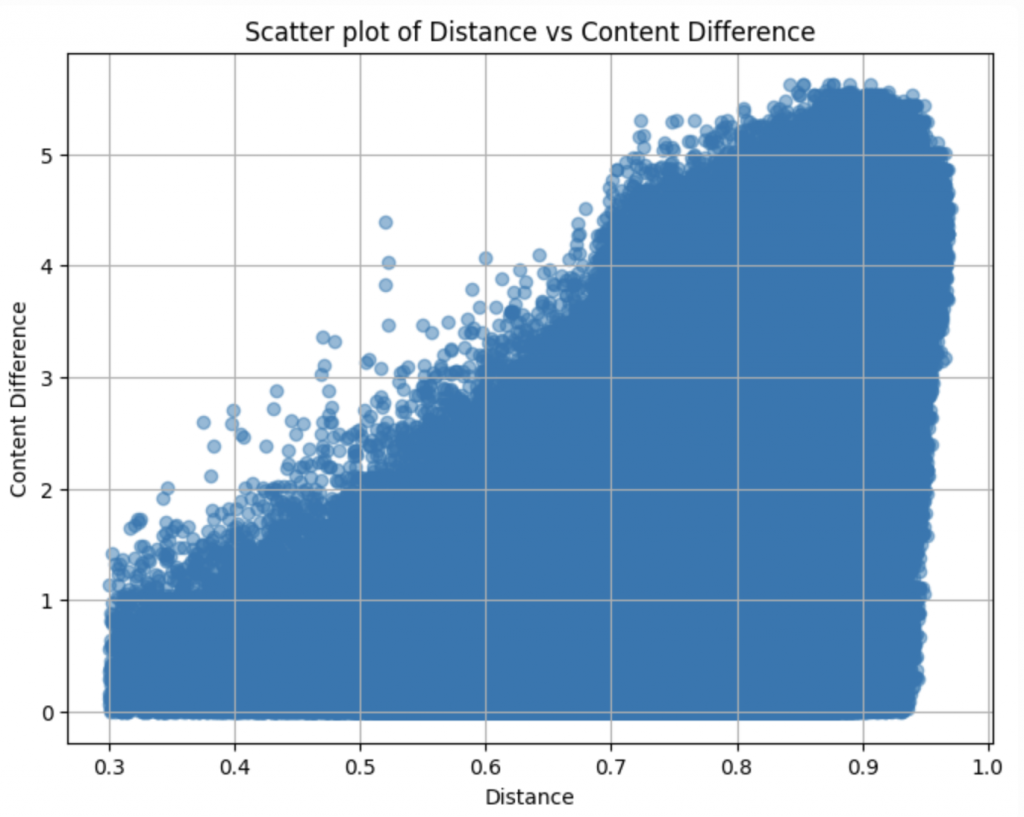
correlation 有到 0.6 左右，代表我們之後在找 feature 的時候，當前data在 trainset 的最近鄰，也許可以成為一個有用的 feature!
因為如果可以在 trainset 中找到和當前這筆 test data 相近內容的摘要，我們就可以假設 test data 最後得到的分數應該和這筆摘要差不太多！

LGBM Baseline 小試身手

到目前為止，我們已經挖掘到一些和 content 與 wording score 非常相關的 feature 了，包含：摘要的字數、摘要與原文的相似度(rougeL, embedding cosine similarity)，還有今天發現的我們可以從訓練資料找最近鄰(nearest neighbor)來當作另外一個 feature 等等。

有了 feature，我們就可以用 LightGBM 作為我們的模型進行初步嘗試！

什麼是 LGBM？

LGBM 是 LightGBM（Light Gradient Boosting Machine）的縮寫，它是一種基於決策樹的梯度提升框架，由微軟開發，特別適合在大規模數據集上進行快速、準確的模型訓練。

LightGBM 屬於梯度提升樹(Gradient Boosting Decision Trees, GBDT)的一種實現，即通過逐步生成多棵決策樹，並且每一棵樹都會學習和修正前一棵樹的誤差，它專注於通過加速和減少內存使用來優化性能。相比其他 GBDT 的實現（如 XGBoost），LightGBM 具有更快的速度和更低的內存占用，尤其在大規模數據集上有顯著的表現。

在 Kaggle 比賽中，選手們常使用 LGBM，主要原因包括：

• 速度快： LGBM 在處理大規模數據集和高維數據時，比其他 GBDT 工具（如 XGBoost）更快。這對於需要反覆調參、優化的比賽來說非常重要。

• 內存占用低： 由於 LGBM 的高效內存使用，在應對數據量非常大的競賽中尤為出色。

• 支持類別型特徵： LGBM 可以原生處理類別型特徵（categorical features），無需像其他工具那樣進行額外的特徵編碼操作，這使得數據處理更為簡便。

• 精度高： 基於其高效的葉子增長方式，LGBM 能在較短時間內達到很高的準確率和良好的泛化能力。

• 靈活性： LGBM 支持大量的參數調整，能夠根據不同的問題場景進行靈活的設置，使其在 Kaggle 比賽中的應用更加廣泛。

在開始前我們可以先從 commonlit 的官網上撈到關於每個題目（prompt）更詳細的介紹，包含這些題目 prompt 分別是給哪些年級的作業等等。我們把這些資訊和 prompt_train 合併起來，組成新的 prompt_train 等等會用到：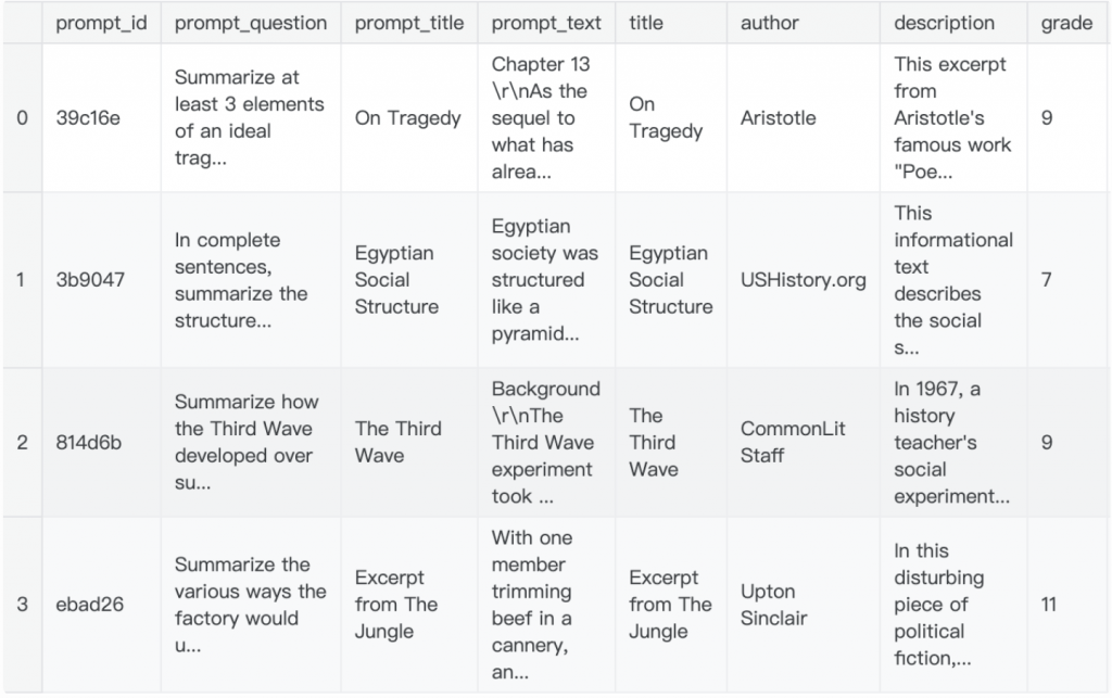

接下來開始處理特徵的部分。

除了上述提到的 feature，我們可以再手動增加一些 feature 讓模型的判斷依據更豐富一些，這些 feature 有些是我們前面沒有討論過的，有些可能會對預測 content/wording score 很有幫助，有些可能沒有。

但沒關係，我希望可以藉由下面的例子帶大家 run 一次我們在產生文本特徵時，有哪些經常會被提及的項目～（以下代碼改寫自 1）

以下是我們會輸入的特徵：

文本長度與分詞

prompt_length: 原文的長度（以詞元計）。
summary_length: 摘要的長度（以詞元計）。
prompt_tokens: 原文的分詞形式。
summary_tokens: 摘要的分詞形式。

拼寫與語法(應該滿容易想到的，如果錯字很多，老師就會扣分)

splling_err_num: 摘要中的拼寫錯誤數量。
gunning_fog, flesch_kincaid_grade_level, flesch_reading_ease: 提示和摘要的可讀性評分。

Lingustic 特徵

word_count, sentence_length, vocabulary_richness: 基本文本統計信息。
avg_word_length, comma_count, semicolon_count: 額外的語言特征。
pos_ratios: 文本中詞性的比例。
punctuation_ratios: 標點符號的比例。

文本相似度與重疊

word_overlap_count, bigram_overlap_count, trigram_overlap_count: 提示與摘要之間的N-gram重疊次數。
jaccard_similarity: 提示與摘要之間的Jaccard相似度。
text_similarity: 自定義文本相似度指標。

情感分析

sentiment_polarity, sentiment_subjectivity: 情感極性和主觀性得分。
sentiment_scores: 詳細的情感得分，進一步分解為單獨的列。

接下來我們可以寫一個 preprocessor 把 train_df 和 test_df 的每個 row 都新增這些我們手動計算的特徵：
代碼中有加入註釋詳細解釋該個特徵是什麼、怎麼被計算的：

• Preprocessor

class Preprocessor:
    def __init__(self, model_name: str) -> None:
        //用來進行文本分詞
        self.tokenizer = AutoTokenizer.from_pretrained(f"/kaggle/input/{model_name}")
        // TreebankWordDetokenizer
        self.twd = TreebankWordDetokenizer()
        // 設置停止詞列表 (STOP_WORDS)，用於過濾掉常見無意義詞語
        self.stop_words = set(stopwords.words('english'))
        // 加載 spaCy 的 NER 模型，用於命名實體識別。
        self.spacy_model = spacy.load('en_core_web_sm')
        // 初始化拼寫檢查器和自動更正器。
        self.spellchecker = SpellChecker()

    // 使用 TfidfVectorizer 計算兩個文本的 TF-IDF 矩陣，並使用餘弦相似度來計算這兩段文本的相似度。
    def calculate_text_similarity(self, row):
        vectorizer = TfidfVectorizer()
        tfidf = vectorizer.fit_transform([row['prompt_text'], row['text']])
        return cosine_similarity(tfidf[0:1], tfidf[1:2]).flatten()[0]
    
    //使用 TextBlob 庫來進行情感分析，返回情感極性和主觀性。
    def sentiment_analysis(self, text):
        analysis = TextBlob(text)
        return analysis.sentiment.polarity, analysis.sentiment.subjectivity

    // 計算 prompt_text 和 summary_text 中的單詞重疊數，過濾掉停止詞後再進行比較。
    def word_overlap_count(self, row):
        prompt_words = set(row['prompt_tokens']) - self.stop_words
        summary_words = set(row['summary_tokens']) - self.stop_words
        return len(prompt_words & summary_words)

    def ngrams(self, tokens, n):
        return [' '.join(ngram) for ngram in zip(*[tokens[i:] for i in range(n)])]
    // 計算 prompt_text 和 summary_text 中 n-gram 的共現數量，並返回相同的 n-gram 個數。
    def ngram_overlap(self, row, n):
        prompt_ngrams = set(self.ngrams(row['prompt_tokens'], n))
        summary_ngrams = set(self.ngrams(row['summary_tokens'], n))
        return len(prompt_ngrams & summary_ngrams)
    // 使用 spaCy 模型對文本進行命名實體識別，並比較 prompt_text 和 summary_text 中的命名實體重疊情況，返回重疊實體的數量。
    def ner_overlap_count(self, row):
        def extract_entities(text):
            doc = self.spacy_model(text)
            return set((ent.text.lower(), ent.label_) for ent in doc.ents)
        
        prompt_ner = extract_entities(row['prompt_text'])
        summary_ner = extract_entities(row['text'])
        return len(prompt_ner & summary_ner)  # 返回重疊的命名實體數量
    // 計算 summary_text 中引用的語句在 prompt_text 中出現的次數。
    def quotes_count(self, row):
        summary = row['text']
        text = row['prompt_text']
        quotes_from_summary = re.findall(r'"([^"]*)"', summary)
        return sum(quote in text for quote in quotes_from_summary) if quotes_from_summary else 0
    // 使用拼寫檢查器來計算文本中的拼寫錯誤數量。
    def spelling_errors(self, text):
        """返回拼寫錯誤的數量"""
        wordlist = text.split()
        return len(list(self.spellchecker.unknown(wordlist)))

    def run(self, prompts: pd.DataFrame, summaries: pd.DataFrame) -> pd.DataFrame:
        # Tokenization
        prompts["prompt_tokens"] = prompts["prompt_text"].apply(word_tokenize)
        summaries["summary_tokens"] = summaries["text"].apply(word_tokenize)
        
        # Merge prompts and summaries
        merged_df = summaries.merge(prompts, on="prompt_id", how="left")
        
        # Features
        merged_df['text_similarity'] = merged_df.apply(self.calculate_text_similarity, axis=1)
        merged_df['word_overlap_count'] = merged_df.apply(self.word_overlap_count, axis=1)
        merged_df['bigram_overlap'] = merged_df.apply(self.ngram_overlap, args=(2,), axis=1)
        merged_df['trigram_overlap'] = merged_df.apply(self.ngram_overlap, args=(3,), axis=1)
        merged_df['ner_overlap_count'] = merged_df.apply(self.ner_overlap_count, axis=1)
        merged_df['quotes_count'] = merged_df.apply(self.quotes_count, axis=1)
        merged_df['spelling_errors'] = merged_df['text'].apply(self.spelling_errors)

        # Sentiment analysis
        merged_df[['sentiment_polarity', 'sentiment_subjectivity']] = merged_df['text'].apply(
            lambda x: pd.Series(self.sentiment_analysis(x))
        )
        
        return merged_df.drop(columns=["summary_tokens", "prompt_tokens"])

• 開始計算 train_df, test_df 的這些 hand_craft 特徵，並連同之前的 column 複製到新的 dataframe

train = preprocessor.run(prompts_train, summaries_train)
test = preprocessor.run(prompts_test, summaries_test)

準備好 train/test data 了，接下來就可以開始訓練模型。
但是這邊我們一樣要做 cross-validation，並且想根據 prompt 的 grade （前面有處理過）來切分 train/valid dataset，所以我們使用 GroupKFold，並且根據 train['grade'] 來切。(train set 共有三個不同年級)

# Calculate the number of unique groups
n_unique_groups = train["grade"].nunique()

# Set n_splits to be the smaller of CFG.n_splits and the number of unique groups
n_splits = min(CFG.n_splits, n_unique_groups)
gkf = GroupKFold(n_splits=n_splits)

for i, (_, val_index) in enumerate(gkf.split(train, groups=train["grade"])):
    train.loc[val_index, "fold"] = i

最後做出來的 train dataset 就會長這樣：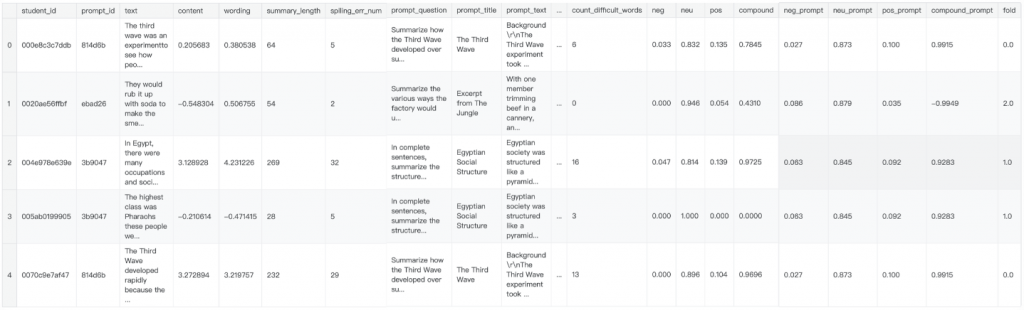

每一筆資料都包含摘要的文字、他摘要的對象也就是原文的資訊，以及摘要與原文一起計算出的各式各樣的 feature，最後一個 column:fold則是代表現在這個資料是在 cross validation 切出來的 n-folds 中，是屬於哪一個 fold。

接下來我們定義一些要計算的評估指標的 function:

def compute_metrics(eval_pred):
    predictions, labels = eval_pred
    rmse = mean_squared_error(labels, predictions, squared=False)
    return {"rmse": rmse}

def compute_mcrmse(eval_pred):
    """
    Calculates mean columnwise root mean squared error
    https://www.kaggle.com/competitions/commonlit-evaluate-student-summaries/overview/evaluation
    """
    preds, labels = eval_pred

    col_rmse = np.sqrt(np.mean((preds - labels) ** 2, axis=0))
    mcrmse = np.mean(col_rmse)

    return {
        "content_rmse": col_rmse[0],
        "wording_rmse": col_rmse[1],
        "mcrmse": mcrmse,
    }

def compt_score(content_true, content_pred, wording_true, wording_pred):
    content_score = mean_squared_error(content_true, content_pred)**(1/2)
    wording_score = mean_squared_error(wording_true, wording_pred)**(1/2)
    
    return (content_score + wording_score)/2

使用Optuna找到最優參數

為了節省我們調參數的負擔，這邊使用Optuna 進行超參數調優。
(註：今天發現今年也有選手特別介紹 Optuna 的用法，寫得很清楚！推薦大家可以過去看看：打鐵趁熱！來試著使用Optuna解決問題吧。看完之後可以想想看，如果要用 Optuna 調整 LGBM 的 learning_rate(range: 0.01~0.1), max_depth(range: 2~10), lambda_l1(range: 1e-8~10)等等參數，該怎麼寫呢？）

首先要先定義我們的 objective function:
下面的 trial 參數就是等一下 Optuna 會傳入的東西，由他來決定下載的 learning rate, max_depth 等等參數。

# 目標函數
def objective(trial, X_train, y_train, X_eval, y_eval):
    params = {
        'boosting_type': 'gbdt',
        'objective': 'regression',
        'metric': 'rmse',
        'learning_rate': trial.suggest_float('learning_rate', 0.01, 0.1),
        'max_depth': trial.suggest_int('max_depth', 2, 10),
        'num_leaves': trial.suggest_int('num_leaves', 2, 2 ** trial.suggest_int('max_depth', 2, 10) - 1),
        'lambda_l1': trial.suggest_loguniform('lambda_l1', 1e-8, 10.0),
        'lambda_l2': trial.suggest_loguniform('lambda_l2', 1e-8, 10.0),
        'random_state': 42,
        'verbosity': -1  # 禁止打印警告
    }

    dtrain = lgb.Dataset(X_train, label=y_train)
    dval = lgb.Dataset(X_eval, label=y_eval)

    # 模型訓練
    model = lgb.train(
        params, dtrain, num_boost_round=10000, valid_sets=[dtrain, dval], 
        valid_names=['train', 'valid'], early_stopping_rounds=30, 
        verbose_eval=1000
    )
    
    trial.set_user_attr('best_model', model)
    return model.best_score['valid']['rmse']  # 返回驗證集上的 RMSE

我們一共有兩個目標變量：

# 目標變量
targets = ["content", "wording"]

針對這兩個 target 在不同 folds 的 data 上找到最優化的參數：

model_dict = {}

# 對每個目標變量進行模型訓練和調參
for target in targets:
    models = []
    
    for fold in range(CFG.n_splits):
        # 分割訓練集和驗證集
        X_train = train[train["fold"] != fold].drop(columns=drop_columns)
        y_train = train[train["fold"] != fold][target]
        X_eval = train[train["fold"] == fold].drop(columns=drop_columns)
        y_eval = train[train["fold"] == fold][target]

        # 使用 Optuna 進行調參
        study = optuna.create_study(direction='minimize')
        study.optimize(lambda trial: objective(trial, X_train, y_train, X_eval, y_eval), n_trials=100)
        
        print(f'Best trial for {target}, fold {fold}: score {study.best_value}, params {study.best_params}')

        # 儲存最佳模型
        best_model = study.best_trial.user_attrs['best_model']
        models.append(best_model)
    
    # 將每個目標變量的模型存入字典
    model_dict[target] = models

到這邊，訓練就結束啦！
之後 inference 的時候就從 model_dict 取出 content 和 wording 的 model list，再取得每一個 model 的預測數值最後做平均即可！或是像下面作者，他計算每一折的模型預測出的結果，取得中位數與標準差之後，將中位數微調當作最後輸出，也是一種 ensemble 的方法～

# 計算 K-Fold 預測的中位數
medians = test[[f'{target}_pred_{fold}' for fold in range(CFG.n_splits)]].median(axis=1)

# 計算 K-Fold 預測的標準差
std_devs = test[[f'{target}_pred_{fold}' for fold in range(CFG.n_splits)]].std(axis=1)

# 使用標準差調整中位數
adjusted_medians = medians + (CFG.adjustment_factor * std_devs)

test[target] = adjusted_medians

小結

可以猜看看，像這樣用一些 hand-craft 的 feature 輸入到 LGBM 訓練，可以在 LB 上排到第幾名呢？

結果是...

Public Score 大概是 0.47 分（這個分數越低越好），排名在 1036，大概排行榜的 50% 左右。

其實好像比想像中好？？

事實上有很多用 BERT, deberta 等語言模型下去訓練的組別，還遠遠排在這個使用 LGBM 模型訓練的方案後面喔！

由於 LGBM 的迭代速度很快，所以很多 Kaggler 會選擇用 LGBM 當作一開始的 baseline，嘗試一些 feature 觀察看看效果之後，再慢慢改進～

除此之外，今天提到的使用Optuna 進行超參數調優，也是不錯的技巧，大家有需要的話，可以參考上面的做法～

明天我們會開始介紹本賽題的前四名優勝解法，其中有一組會利用到今天發現的作弊data的一些性質來改進自己的方法～

那麼，我們明天見！

謝謝讀到最後的你，希望你會覺得有趣！
如果喜歡這系列，別忘了按下訂閱，才不會錯過最新更新，也可以按讚給我鼓勵唷！
如果有任何回饋和建議，歡迎在留言區和我說✨✨

（Kaggle - CommonLit - Evaluate Student Summaries 解法分享系列）