
最後一個關於效能的主題,我們要來看的是在 PostgreSQL 中不同的 JOIN 方式。JOIN 是將多個表的資料關聯起來的方式,而 PostgreSQL 針對不同的查詢場景,提供了多種 JOIN 策略,包括 Nested Loop Join、Hash Join 和 Merge Join。不同的 JOIN 策略會影響查詢的效能。
之前在使用 EXPLAIN ANALAZE 的時候,可能就有觀察到不同 JOIN 出現在 query planner 中。今天的文章就會透過 EXPLAIN ANALYZE 來觀察不同 JOIN 的執行方式,並了解它們的適用情境。
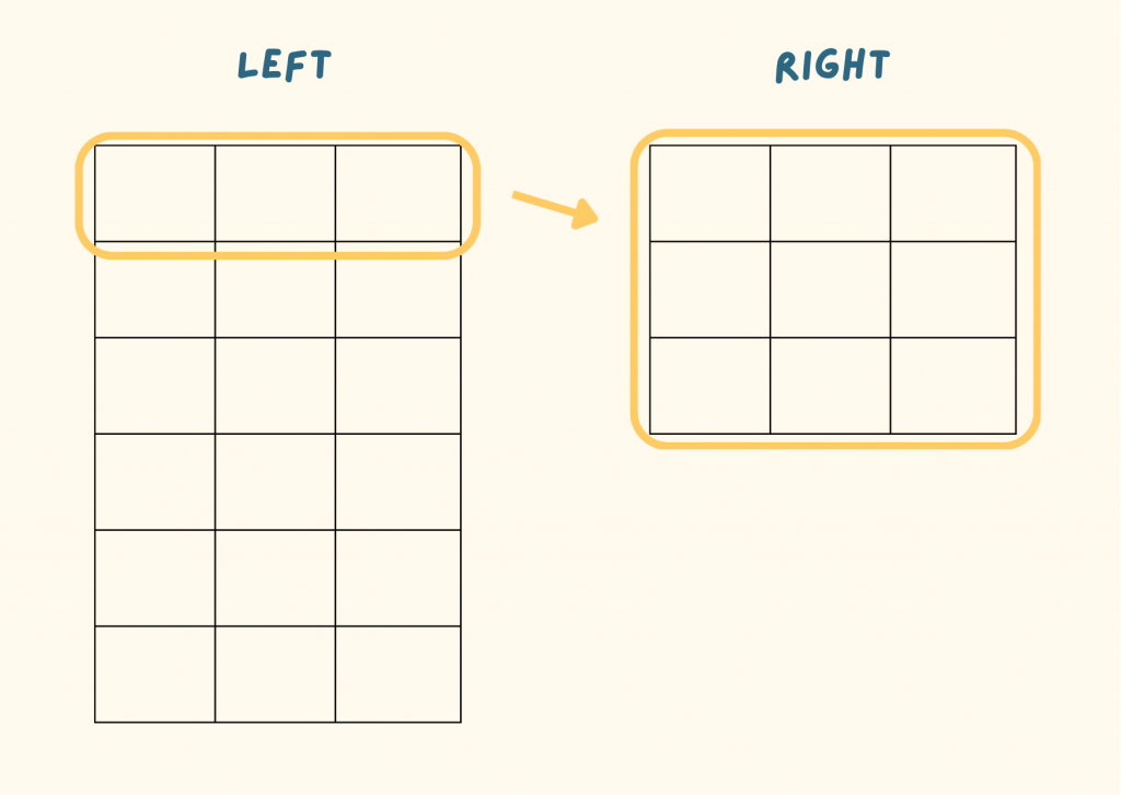
第一個要介紹的是 Nested Loop Join,如果是採用這個方式,PostgreSQL 會對 left attribute 逐行掃描,並使用 JOIN 條件去 right attribute 查找對應的值。這種方式對於小表 JOIN 大表且 right attribute 有 Index 的情境效率較好。
觀察 Nested Loop Join
情境:小表 JOIN 大表且 right attribute 有 Index
departments 可以被當作小表,employees 是大表CREATE TABLE departments (
department_id SERIAL PRIMARY KEY,
department_name VARCHAR(100),
location VARCHAR(100)
);
CREATE TABLE employees (
employee_id SERIAL PRIMARY KEY,
department_id INT,
first_name VARCHAR(50),
last_name VARCHAR(50),
email VARCHAR(100)
);
departments (小表 5 筆資料)departments = [
("Human Resources", "New York"),
("Engineering", "San Francisco"),
("Marketing", "Chicago"),
("Sales", "Los Angeles"),
("Finance", "Boston"),
]
cursor.executemany(
"""
INSERT INTO departments (department_name, location)
VALUES (%s, %s)
""",
departments,
)
employees(大表 10000 筆資料)employee_data = []
for _ in range(10000):
first_name = fake.first_name()
last_name = fake.last_name()
email = f"{first_name.lower()}.{last_name.lower()}@company.com"
employee_data.append(
(
random.randint(1, 5), # 隨機分配一個 department
first_name,
last_name,
email,
)
)
cursor.executemany(
"""
INSERT INTO employees (department_id, first_name, last_name, email)
VALUES (%s, %s, %s, %s)
""",
employee_data,
)
EXPLAIN ANALYZE
SELECT * FROM departments d
JOIN employees e ON d.department_id = e.department_id
WHERE d.department_id = 1;
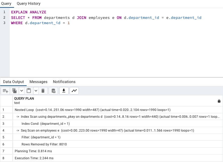
因為 departments 資料較少,employees 資料較多,employees 可以當成 left attribute,逐行掃描後用 department_id 去找對應的資料。
而且 departments 的 department_id 有 Index (Primary key),所以還可以看到是使用 Index Scan 讓查詢速度更快。也對應到文件上所說的,想象中逐一掃描 employees 的每一行對應 departments 的哪一個位置好像會很費時,但如果對應的欄位能夠 Index Scan,那這就是一個適合的策略。
The right relation is scanned once for every row found in the left relation. This strategy is easy to implement but can be very time consuming. (However, if the right relation can be scanned with an index scan, this can be a good strategy. It is possible to use values from the current row of the left relation as keys for the index scan of the right.)
第二種方法是 Hash Join ,Hash Join 會先掃描 right attribute,將 key-value 組成 Hash Table 儲存在記憶體中。接著掃描左表並使用 Hash Table 來查找對應值。通常發生在大表 JOIN 大表,但沒有 Index 的情況。
The right relation is first scanned and loaded into a hash table, using its join attributes as hash keys. Next the left relation is scanned and the appropriate values of every row found are used as hash keys to locate the matching rows in the table.
沒有 Index 所以將右表變成 Hash Table,左表在比對的時候才能找得比較快:
| Key | Value |
|---|---|
| 1 | {"department_id": 1, "department_name": "Human Resources", "location": "New York"} |
| 2 | {"department_id": 2, "department_name": "Engineering", "location": "San Francisco"} |
| 3 | {"department_id": 3, "department_name": "Marketing", "location": "Chicage"} |
| 4 | {"department_id": 4, "department_name": "Sales", "location": "Los Angeles"} |
| 5 | {"department_id": 5, "department_name": "Finance", "location": "Boston"} |
觀察 Hash Join
情境:大表 JOIN 大表,但沒有 Index
CREATE TABLE orders(
	id INT,
	final_status TEXT
);

CREATE TABLE order_history(
	id INT,
	status TEXT
);
# orders 塞入 10000 筆資料
customers = [
    (i, fake.random_element(elements=("pending", "completed", "cancelled")))
    for i in range(1, 10001)
]

cursor.executemany(
    """
    INSERT INTO orders (id, final_status) VALUES (%s, %s)
""",
    customers,
)

# order history 塞入 10000 筆資料
orders = [
    (
        i,
        fake.random_element(elements=("pending", "completed", "cancelled")),
    )
    for i in range(1, 10001)
]
cursor.executemany(
    """
    INSERT INTO order_history (id, status) VALUES (%s, %s)
""",
    orders,
)
EXPLAIN ANALYZE
SELECT *
FROM public.orders
JOIN public.order_history
ON orders.id = order_history.id;
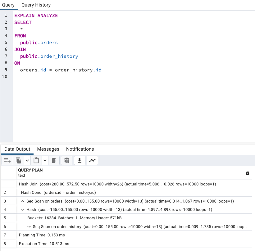
因為 orders 和 order_history 沒有 Index,因此 PostgreSQL 在這裡選擇 Hash Join。
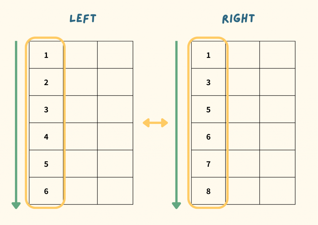
第三個方法是 Merge Join ,Merge Join 會先對兩張 table JOIN 條件的欄位進行排序,然後比對及合併兩張表。適用於兩張表都已排序或有 Index、大表 JOIN 大表且有 Index。
Each relation is sorted on the join attributes before the join starts. Then the two relations are scanned in parallel, and matching rows are combined to form join rows. This kind of join is attractive because each relation has to be scanned only once. The required sorting might be achieved either by an explicit sort step, or by scanning the relation in the proper order using an index on the join key.
觀察 Merge Join
情境:兩張表都已排序或有 Index、大表 JOIN 大表且有 Index
CREATE INDEX idx_orders_id ON orders(id);
CREATE INDEX idx_order_history_id ON order_history(id);
EXPLAIN ANALYZE
SELECT *
FROM public.orders
JOIN public.order_history
ON orders.id = order_history.id
ORDER BY orders.id, order_history.id; -- 加上排序的選項
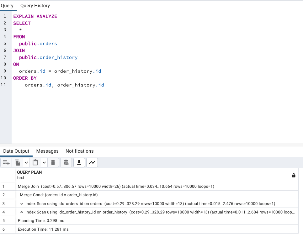
發現這裡的 orders.id 和 order_history.id 都有 Index 後,資料庫能直接利用它來取得已排序的結果,所以接著只要再使用 Merge Join 來得到最終的資料。
EXPLAIN ANALYZE 來分析 query plan,可以了解 PostgreSQL 選擇的 JOIN 策略。https://www.postgresql.org/docs/current/planner-optimizer.html#PLANNER-OPTIMIZER-GENERATING-POSSIBLE-PLANS
https://gelovolro.medium.com/what-are-merge-join-hash-join-and-nested-loop-example-in-postgresql-29123ca18fd1

 iThome鐵人賽