今天我們要來聊聊 LLM 的微調技巧。因為 Whisper 是一個參數量非常大的模型,所以我們會簡單介紹一下什麼是 QLoRA,還有怎麼在程式裡面進行量化,並轉換成 QLoRA 的格式。那就讓我們一起來看看,要怎麼微調一個中文的 ASR Whisper 模型吧。
QLoRA(Quantized Low-Rank Adaptation)是一種專為大型語言模型設計的高效微調技術,旨在顯著降低訓練過程中的參數量與計算成本。它巧妙地結合了量化(Quantization)與低秩適應(Low-Rank Adaptation)兩種方法,實現了資源節省與模型表現之間的平衡。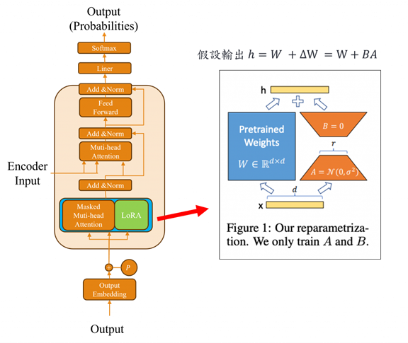
QLoRA 的核心作法是在將原始神經網路進行量化並凍結其參數後,額外加上一個外掛模組 Adapter(適配器)。這樣的設計背後有其必要性,由於模型權重經過量化,從高精度格式(如 float64)轉為較低精度(如 float32 甚至更低),雖然顯著降低了記憶體消耗,卻也可能犧牲部分精度。為了補償這種潛在損失,Adapter 被用來模擬參數更新的能力,使模型在保持輕量的同時,仍能維持良好的學習與泛化效果。這種策略不僅提升了微調效率,也大幅擴展了大型模型在資源受限環境中的應用潛力。
我們首先使用 BitsAndBytesConfig 來設定量化相關的參數。這次選擇的是 4-bit 量化,也就是將模型中的部分浮點數權重轉換成更小的格式,以此降低記憶體的使用量。
quant_config = BitsAndBytesConfig(
    load_in_4bit=True,  # 啟用 4-bit 量化
    bnb_4bit_compute_dtype=torch.float16,  # 運算時用 float16,速度與精度兼顧
    bnb_4bit_use_double_quant=True,  # 啟用雙層量化,進一步壓縮
    bnb_4bit_quant_type='nf4'  # 使用 nf4(Normalized Float 4)作為量化方式
)
接下來我們載入 whisper-large-v3-turbo 模型,並將前面設定好的量化參數套用到模型中。這個過程非常簡單,只需要將設定好的參數作為引數傳入即可。
base_model = AutoModelForSpeechSeq2Seq.from_pretrained(
    'openai/whisper-large-v3-turbo',
    quantization_config=quant_config,
    torch_dtype=torch.float16,
    use_cache=False
)
如果我們 print 出模型結構,可以發現許多原本的 Linear 層已經被替換成了 Linear4bit。這代表這些層的權重如今都已經轉換成 4-bit 格式起來會像這樣:
WhisperForConditionalGeneration(
  (model): WhisperModel(
    (encoder): WhisperEncoder(
      (conv1): Conv1d(128, 1280, kernel_size=(3,), stride=(1,), padding=(1,))
      (conv2): Conv1d(1280, 1280, kernel_size=(3,), stride=(2,), padding=(1,))
      (embed_positions): Embedding(1500, 1280)
      (layers): ModuleList(
        (0-31): 32 x WhisperEncoderLayer(
          (self_attn): WhisperSdpaAttention(
            (k_proj): Linear4bit(in_features=1280, out_features=1280, bias=False)
            (v_proj): Linear4bit(in_features=1280, out_features=1280, bias=True)
            (q_proj): Linear4bit(in_features=1280, out_features=1280, bias=True)
            (out_proj): Linear4bit(in_features=1280, out_features=1280, bias=True)
          )
          (self_attn_layer_norm): LayerNorm((1280,), eps=1e-05, elementwise_affine=True)
          (activation_fn): GELUActivation()
          (fc1): Linear4bit(in_features=1280, out_features=5120, bias=True)
          (fc2): Linear4bit(in_features=5120, out_features=1280, bias=True)
          (final_layer_norm): LayerNorm((1280,), eps=1e-05, elementwise_affine=True)
        )
      )
      (layer_norm): LayerNorm((1280,), eps=1e-05, elementwise_affine=True)
    )
    (decoder): WhisperDecoder(
      (embed_tokens): Embedding(51866, 1280, padding_idx=50257)
      (embed_positions): WhisperPositionalEmbedding(448, 1280)
      (layers): ModuleList(
        (0-3): 4 x WhisperDecoderLayer(
          (self_attn): WhisperSdpaAttention(
            (k_proj): Linear4bit(in_features=1280, out_features=1280, bias=False)
            (v_proj): Linear4bit(in_features=1280, out_features=1280, bias=True)
            (q_proj): Linear4bit(in_features=1280, out_features=1280, bias=True)
            (out_proj): Linear4bit(in_features=1280, out_features=1280, bias=True)
          )
          (activation_fn): GELUActivation()
          (self_attn_layer_norm): LayerNorm((1280,), eps=1e-05, elementwise_affine=True)
          (encoder_attn): WhisperSdpaAttention(
            (k_proj): Linear4bit(in_features=1280, out_features=1280, bias=False)
            (v_proj): Linear4bit(in_features=1280, out_features=1280, bias=True)
            (q_proj): Linear4bit(in_features=1280, out_features=1280, bias=True)
            (out_proj): Linear4bit(in_features=1280, out_features=1280, bias=True)
          )
          (encoder_attn_layer_norm): LayerNorm((1280,), eps=1e-05, elementwise_affine=True)
          (fc1): Linear4bit(in_features=1280, out_features=5120, bias=True)
          (fc2): Linear4bit(in_features=5120, out_features=1280, bias=True)
          (final_layer_norm): LayerNorm((1280,), eps=1e-05, elementwise_affine=True)
        )
      )
      (layer_norm): LayerNorm((1280,), eps=1e-05, elementwise_affine=True)
    )
  )
  (proj_out): Linear(in_features=1280, out_features=51866, bias=False)
實際上他們的轉換方式大致就是透過類似下面這樣的步驟,逐一將模型中的每個 nn.Linear 層替換成對應的 Linear4bit 模組。這裡的 Linear4bit 跟 PyTorch 裡常用的 nn.Linear 最大的差別就是它的權重格式不同。nn.Linear 使用的是 float32 或 float16,而 Linear4bit 則是使用更壓縮的 4-bit 格式,就是你把原本用 float32 的大胖模型換成了壓縮過的瘦身模型,跑起來比較快、佔的記憶體也少,對部署來說非常實用。
我們現在要做的事情,是讓一個大型語言模型準備好進行低位元量化訓練(k-bit training)。這個做法可以大幅節省記憶體、提升訓練效率,特別是在 GPU 資源有限的情況下非常實用。而這裡的關鍵步驟就是使用 prepare_model_for_kbit_training 這個方法。這個函式會幫我們做幾件很重要的事情,來讓模型進入可訓練、可量化的狀態:
啟用 gradient checkpointing 時,系統預設會啟用以下幾項優化策略,首先模型在前向傳播階段通常會保留每一層的中間值(activations),以便於後續的反向傳播。不過當啟用 gradient checkpointing 後,僅會儲存關鍵節點的中間值,其餘部分則在反向傳播時再動態重新計算,以節省記憶體。
其次為了避免不必要的運算資源浪費,系統會自動凍結那些不需要參與訓練的參數,例如 LayerNorm 或 embedding 層中原本就不打算更新的部分。最後還會根據執行環境,自動設定資料型別(dtype)與運算設備(device),進一步提升執行效率與穩定性。
# 準備模型支援量化訓練
base_model = prepare_model_for_kbit_training(base_model, use_gradient_checkpointing=False)
接著我們建立一個 LoRA 訓練的設定檔,這個設定檔會指定:
from peft import (
    LoraConfig,
    get_peft_model,
    prepare_model_for_kbit_training,
)

# 建立 LoRA 配置
lora_config = LoraConfig(
    r=8,
    lora_alpha=16,
    lora_dropout=0.05,
    bias='none',
    target_modules=['q_proj', 'v_proj']
)
當我們用 get_peft_model 這個函式時,其實就是在模型上加上像 LoRA 或其他 PEFT 的層,讓它可以被訓練。它會根據你給的 peft_config 插入像 LoRA 這種 adapter 模組,然後把這些 adapter 設定成可訓練的,其他原本的模型參數就會被凍結起來不動。這樣一來只訓練 adapter 的部分,就可以達到快速又節省資源的微調效果。
# 加入 LoRA 模型
model = get_peft_model(base_model, lora_config)
接下來我們需要從 GitHub 下載這次要用的資料集,下載完之後我們會用 librosa 這個音訊處理套件來讀取音檔。
在讀取的時候,有兩個重要的設定要注意:
sr=16000:這表示我們把音檔的取樣率(sampling rate)設成 16kHz。這個設定在語音處理領域非常常見,尤其是像 Whisper 這樣的語音辨識模型,它要求輸入的音訊一定得是 16kHz,否則模型無法正確處理。透過這個參數,我們可以在讀取時直接把音檔轉換成 16kHz,確保後續處理流程順利進行。mono=True:這表示不管原始音檔是單聲道還是立體聲,我們都會把它轉成單聲道(mono),這樣處理起來比較一致也省記憶體。librosa 幫我們讀音檔,確保格式是統一的、適合後面模型使用。import os
import pandas as pd
import librosa
from tqdm import tqdm
def load_dataset(audio_dir, transcript_file='ASR_CN.csv', target_sr=16000):
df = pd.read_csv(transcript_file, encoding='utf-8-sig')
df['path'] = df['ID'].apply(lambda x: os.path.join(audio_dir, x))
print(f'>>> 共有 {len(df)} 筆紀錄,開始載入音訊...')
audio_list = []
sentence_list = []
for _, row in tqdm(df.iterrows(), total=len(df), desc="載入音訊中", unit="記錄"):
wav_path = row['path']
sentence = row.get('sentence', '').strip()
audio, sr = librosa.load(wav_path, sr=target_sr, mono=True)
audio_list.append(audio)
sentence_list.append(sentence)
return audio_list, sentence_list
audios, sentences = load_dataset('audio', 'ASR_CN.csv', target_sr=16000)
在 Whisper 模型中,WhisperProcessor 是專門設計來處理語音資料的工具,它融合了特徵擷取(feature extraction)和 tokenizer 的功能。在 Whisper 中不直接處理聲音波形(raw waveform),而是透過 WhisperFeatureExtractor 將聲音轉換成對應的對數梅爾頻譜圖(log-Mel spectrogram)。這個格式能保留語音的音高與語調特徵,是模型理解聲音的基礎。
在Whisper 的 tokenizer 會在輸入序列中加上特定的控制 token,這些 token 讓模型知道它要做什麼任務、處理哪種語言、是否需要加入標點或時間戳。例如:
<|en|>:代表這段語音是英文。<|transcribe|>:代表這是語音轉文字(ASR)任務。<|notimestamps|>:指示模型不要在輸出中加入時間戳。<|startoftranscript|>:代表轉錄的開始。<|endoftext|>:代表文本結束。像是如果我們要告訴模型:「我要開始轉錄英文語音,任務是語音轉文字,請不要加時間戳。」可以這樣撰寫
input_tokens = ["<|startoftranscript|>", "<|en|>", "<|transcribe|>", "<|notimestamps|>"]
而模型對應的輸出則會像是
output_tokens = ["▁Hello", "▁world", "!", "<|endoftext|>"]
其中 ▁ 是空格的標記(代表 subword tokenization),而 <|endoftext|> 告訴系統這是文本結尾。而這些Token我們可以直接在一開始就使用AutoProcessor進行設定。
from transformers import AutoProcessor

processor = AutoProcessor.from_pretrained(
    'openai/whisper-large-v3-turbo',
    predict_timestamps=False,
    task="transcribe",
    language='zh'
)
Whisper 模型在輸入的時候,需要三樣東西:
from torch.utils.data import Dataset, DataLoader

class SpeechSeq2SeqDataset(Dataset):

    def __init__(self, input_features, attention_masks, sentences, processor):
        assert len(input_features) == len(attention_masks) == len(sentences)
        self.input_features = input_features
        self.attention_masks = attention_masks
        self.sentences = sentences
        self.processor = processor

    def __len__(self):
        return len(self.input_features)

    def __getitem__(self, idx):
        return {
            "input_features": self.input_features[idx],
            "attention_mask": self.attention_masks[idx],
            "sentence": self.sentences[idx],
        }

    def collate_fn(self, batch):
        input_feats = torch.stack([item['input_features'] for item in batch])
        attention_masks = torch.stack([item['attention_mask'] for item in batch])
        sentences = [item['sentence'] for item in batch]

        # 處理 target:tokenizer 編碼句子
        tok = self.processor.tokenizer(
            sentences,
            padding=True,
            return_tensors='pt',
            return_attention_mask=True
        )

        # 對非 padding 的部分保留,其他設為 -100 以供 loss 使用
        labels = tok['input_ids'].masked_fill(tok['attention_mask'].ne(1), -100)

        return {
            'input_features': input_feats,
            'attention_mask': attention_masks,
            'labels': labels
        }


from sklearn.model_selection import train_test_split

# 拆分資料
feat_train, feat_valid, attn_train, attn_valid, sent_train, sent_valid = train_test_split(
    input_features, attention_mask, sentences, train_size=0.8, random_state=2526, shuffle=True
)

# 建立 Dataset
train_dataset = SpeechSeq2SeqDataset(feat_train, attn_train, sent_train, processor)
valid_dataset = SpeechSeq2SeqDataset(feat_valid, attn_valid, sent_valid, processor)

# DataLoader
train_loader = DataLoader(train_dataset, batch_size=4, shuffle=True, collate_fn=train_dataset.collate_fn)
valid_loader = DataLoader(valid_dataset, batch_size=4, shuffle=False, collate_fn=valid_dataset.collate_fn)
在寫程式的邏輯上其實跟我們用 GPT 的時候滿像的。先在 collate_fn 裡把語音的特徵跟 attention mask 疊成一個 batch,然後把文字丟給 tokenizer 把它轉成數字。為了讓模型專心學有意義的部分,我們會把 padding 的地方設成 -100,這樣在算 loss 的時候就會自動跳過那些沒內容的地方。
同樣的這次整合了 AdamW 優化器與 cosine warmup 學習率調整策略。但要記得 is_lora=True 時,表示模型啟用了 LoRA 格式。在此設定下若使用舊有的模型儲存方式,將會導致錯誤,因此必須使用與 LoRA 相容的保存與載入方式。
from trainer import Trainer
import torch.optim as optim
from transformers import get_cosine_schedule_with_warmup

# 總步數 = epoch 數 * 每個 epoch 的 batch 數
num_training_steps = len(train_loader) * 100  # 100 是總 epoch 數
num_warmup_steps = int(0.2 * len(train_loader))  # 可調整 warmup 比例

optimizer = optim.AdamW(model.parameters(), lr=1e-4)
scheduler = get_cosine_schedule_with_warmup(
    optimizer,
    num_warmup_steps=num_warmup_steps,
    num_training_steps=num_training_steps,
)
trainer = Trainer(
    epochs=100,
    train_loader=train_loader,
    valid_loader=valid_loader,
    model=model,
    optimizer=optimizer,
    scheduler=scheduler,
    early_stopping=5,
    load_best_model=True,
    grad_clip=1.0,
    is_lora=True
)

trainer.train(show_loss=True)
輸出結果:
Train Epoch 5: 100%|██████████| 200/200 [02:35<00:00,  1.28it/s, loss=0.123]
Valid Epoch 5: 100%|██████████| 50/50 [00:15<00:00,  3.13it/s, loss=0.611]
Train Loss: 0.24830 | Valid Loss: 0.54996 | Best Loss: 0.51839

Train Epoch 6: 100%|██████████| 200/200 [02:36<00:00,  1.28it/s, loss=0.061]
Valid Epoch 6: 100%|██████████| 50/50 [00:15<00:00,  3.13it/s, loss=0.600]
Train Loss: 0.21451 | Valid Loss: 0.56744 | Best Loss: 0.51839

Train Epoch 7: 100%|██████████| 200/200 [02:36<00:00,  1.28it/s, loss=0.048]
Valid Epoch 7: 100%|██████████| 50/50 [00:15<00:00,  3.14it/s, loss=0.601]
Train Loss: 0.18471 | Valid Loss: 0.58050 | Best Loss: 0.51839
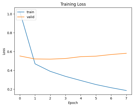
在訓練過程中模型的訓練損失初期較高,約為 1.0,但隨著訓練推進損失穩定下降。到了第 7 個 epoch,訓練損失已降至約 0.2,顯示模型對訓練資料的擬合能力明顯提升。但驗證損失的變化趨勢則有所不同:儘管初期從約 0.55 降至 0.5 左右,之後卻出現逐步上升,特別是在第 4 到第 7 個 epoch 間,上升趨勢更加明顯。這現象暗示模型在驗證資料上的泛化能力開始退化,代表出現過度擬合。這種情況在預訓練模型中相當常見,反映出這類模型即便在小資料集上也能迅速學習特定模式,卻也因此更容易過度擬合。
好啦今天的 Whisper 介紹就先告一段落啦,也代表你現在已經掌握 Transformer 的架構,還有預訓練模型的基本概念了。不簡單欸。今天我們也小小地踏進了 LLM 的微調世界,學了一種滿基礎但超實用的方法,叫做 LoRA。
那明天呢,我們來輕鬆一點,聊聊什麼是 prompt。不同的 prompt 類型又有什麼差別?我會慢慢帶你看,從最早的 prompt 到現在這些花招百出的技巧,它們是怎麼一步一步演進而來的。
我點擊了 "3. 載入資料" 的連結,沒有看到資料集耶。
抱歉我在撰寫文章後不小心忘記將程式碼上傳,這是正確的 GitHub Repo 連結:https://github.com/AUSTIN2526/learning-wx-b-in-30-days


 iThome鐵人賽