參考網站1 參考網站2

接下來照著R語言使用者的python筆記實作練習！來初步了解整個流程，祥細步驟的意義明後天再來認識～

先將MNIST資料讀入

import tensorflow as tf
from tensorflow.examples.tutorials.mnist import input_data

# 讀入 MNIST
mnist = input_data.read_data_sets("MNIST_data/", one_hot = True)
x_train = mnist.train.images
y_train = mnist.train.labels
x_test = mnist.test.images
y_test = mnist.test.labels

# 設定參數
logs_path = 'TensorBoard/'
n_features = x_train.shape[1]
n_labels = y_train.shape[1]

依樣將過程放入TensorBoard來顯示

# 設定參數
logs_path = 'TensorBoard/'
n_features = x_train.shape[1]
n_labels = y_train.shape[1]

接下來定義sees , tf.Seesion()與tf.InteractiveSession()的差別

# 啟動 InteractiveSession
sess = tf.InteractiveSession()
with tf.name_scope('Input'):
    x = tf.placeholder(tf.float32, shape=[None, n_features])
with tf.name_scope('Label'):
    y_ = tf.placeholder(tf.float32, shape=[None, n_labels])

定義一開始的權重跟bias，都給一個小的不為0的初始值。避免神經元掛掉...

# 自訂初始化權重的函數
def weight_variable(shape):
    initial = tf.truncated_normal(shape, stddev=0.1)
    return tf.Variable(initial)

def bias_variable(shape):
    initial = tf.constant(0.1, shape=shape)
    return tf.Variable(initial)

接下來先照著步驟做一遍明天再來學習裡面細節

# 自訂 convolution 與 max-pooling 的函數
def conv2d(x, W):
    return tf.nn.conv2d(x, W, strides=[1, 1, 1, 1], padding='SAME')

def max_pool_2x2(x):
    return tf.nn.max_pool(x, ksize=[1, 2, 2, 1], strides=[1, 2, 2, 1], padding='SAME')

# 第一層是 Convolution 層（32 個神經元），會利用解析度 5x5 的 filter 取出 32 個特徵，然後將圖片降維成解析度 14x14
with tf.name_scope('FirstConvolutionLayer'):
    W_conv1 = weight_variable([5, 5, 1, 32])
    b_conv1 = bias_variable([32])
    x_image = tf.reshape(x, [-1, 28, 28, 1])
    h_conv1 = tf.nn.relu(conv2d(x_image, W_conv1) + b_conv1)
    h_pool1 = max_pool_2x2(h_conv1)

# 第二層是 Convolution 層（64 個神經元），會利用解析度 5x5 的 filter 取出 64 個特徵，然後將圖片降維成解析度 7x7
with tf.name_scope('SecondConvolutionLayer'):
    W_conv2 = weight_variable([5, 5, 32, 64])
    b_conv2 = bias_variable([64])
    h_conv2 = tf.nn.relu(conv2d(h_pool1, W_conv2) + b_conv2)
    h_pool2 = max_pool_2x2(h_conv2)

# 第三層是 Densely Connected 層（1024 個神經元），會將圖片的 1024 個特徵攤平
with tf.name_scope('DenselyConnectedLayer'):
    W_fc1 = weight_variable([7 * 7 * 64, 1024])
    b_fc1 = bias_variable([1024])
    h_pool2_flat = tf.reshape(h_pool2, [-1, 7 * 7 * 64])
    h_fc1 = tf.nn.relu(tf.matmul(h_pool2_flat, W_fc1) + b_fc1)

Dropout 避免overfitting的方式，有時會砍掉幾個神經元再重train。讓某個神經元權重不要太大

# 輸出結果之前使用 Dropout 函數避免過度配適
with tf.name_scope('Dropout'):
    keep_prob = tf.placeholder(tf.float32)
    h_fc1_drop = tf.nn.dropout(h_fc1, keep_prob)

這裡就是全層連接了，決定0~9哪個數字機率最大。

# 第四層是輸出層（10 個神經元），使用跟之前相同的 Softmax 函數輸出結果
with tf.name_scope('ReadoutLayer'):
    W_fc2 = weight_variable([1024, 10])
    b_fc2 = bias_variable([10])
    y_conv = tf.matmul(h_fc1_drop, W_fc2) + b_fc2

開始training!

# 訓練與模型評估
with tf.name_scope('CrossEntropy'):
    cross_entropy = tf.reduce_mean(tf.nn.softmax_cross_entropy_with_logits(y_conv, y_))
    tf.summary.scalar("CrossEntropy", cross_entropy)
train_step = tf.train.AdamOptimizer(1e-4).minimize(cross_entropy)
correct_prediction = tf.equal(tf.argmax(y_conv,1), tf.argmax(y_,1))
with tf.name_scope('Accuracy'):
    accuracy = tf.reduce_mean(tf.cast(correct_prediction, tf.float32))
    tf.summary.scalar("Accuracy", accuracy)

# 初始化
sess.run(tf.global_variables_initializer())

# 將視覺化輸出
merged = tf.summary.merge_all()
writer = tf.summary.FileWriter(logs_path, graph = tf.get_default_graph())

for i in range(20000):
    batch = mnist.train.next_batch(50)
    if i%100 == 0:
        train_accuracy = accuracy.eval(feed_dict = {x: batch[0], y_: batch[1], keep_prob: 1.0})
        print("step %d, training accuracy %g"%(i, train_accuracy))
        summary = sess.run(merged, feed_dict = {x: batch[0], y_: batch[1], keep_prob: 1.0})
        writer.add_summary(summary, i)
        writer.flush()
    train_step.run(feed_dict={x: batch[0], y_: batch[1], keep_prob: 0.5})

print("test accuracy %g"%accuracy.eval(feed_dict = {x: x_test, y_: y_test, keep_prob: 1.0}))

# 關閉 session
sess.close()

發現準確率來到了99.14% 比先前又升很高的程度了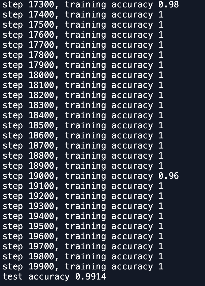

明天再來詳細了解裡面的意義～