前言

上次介紹用來辨識的CNN，這次要介紹影像風格轉換，而這裡使用[2]所介紹到的VGG19模型來訓練，順便練習一下如何載入訓練好的模型。而使用訓練好的模型特徵也稱為遷移學習。

VGG19

首先先了解VGG19的結構，如下圖的E即是VGG19結構，可知道每一層都是使用3X3捲積，池化則是2X2。接著使用Tensorflow讀取已訓練好的VGG19資料。(mat格式)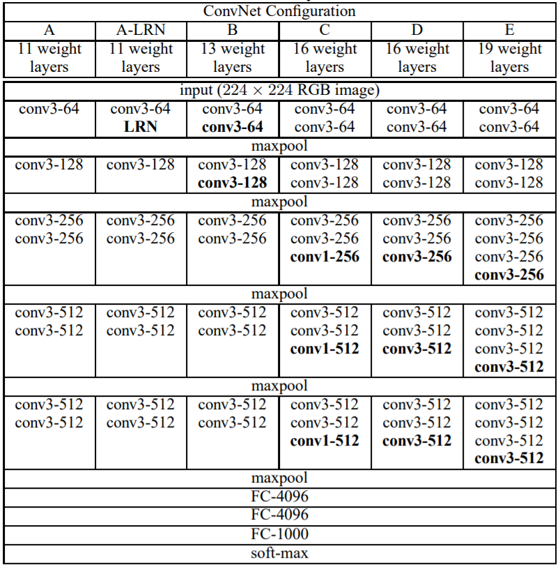

圖來源:[3]。

程式碼

這裡要注意的地方則是np.transpose(weights, [1, 0, 2, 3])，因為mat儲存格式為[width, height, in_channels, out_channels]而Tensorflow計算格式為[height, width, in_channels, out_channels]所以必須要轉置矩陣到對應位置。

• layers為每一層名稱。
• VGG19_build為讀取資料函數，參數vgg19_path為mat檔案路徑，image_data為影像資料，回傳權重型態為Tensor的陣列。
• conv2d為回傳計算3X3捲積。
• max_pool為回傳計算2X2池化。
• relu為回傳relu活化函數。

import tensorflow as tf
import numpy as np
import scipy.io

layers = (
        'conv1_1', 'relu1_1', 'conv1_2', 'relu1_2', 'pool1',
        'conv2_1', 'relu2_1', 'conv2_2', 'relu2_2', 'pool2',
        'conv3_1', 'relu3_1', 'conv3_2', 'relu3_2', 'conv3_3',
        'relu3_3', 'conv3_4', 'relu3_4', 'pool3',
        'conv4_1', 'relu4_1', 'conv4_2', 'relu4_2', 'conv4_3',
        'relu4_3', 'conv4_4', 'relu4_4', 'pool4',
        'conv5_1', 'relu5_1', 'conv5_2', 'relu5_2', 'conv5_3',
        'relu5_3', 'conv5_4', 'relu5_4'
    )

def VGG19_build(vgg19_path, image_data):
    mat_data = scipy.io.loadmat(vgg19_path)
    layers_data = mat_data['layers'][0]

    nets = {}
    output = image_data
    for index, name in enumerate(layers):
        kind = name[:4]
        if kind == 'conv':
            weights, biases = layers_data[index][0][0][0][0]
            # mat: weights 格式依序為[width, height, in_channels, out_channels]
            # tensorflow: weights 格式依序為[height, width, in_channels, out_channels]
            weights = np.transpose(weights, [1, 0, 2, 3])
            biases = biases.reshape(-1)
            output = conv2d(output, weights, biases)
        elif kind == 'relu':
            output = relu(output)
        elif kind == 'pool':
            output = max_pool(output)

        nets[name] = output

    return nets
    

def conv2d(input, weights, biases):
    conv = tf.nn.conv2d(input, tf.constant(weights), strides=[1, 1, 1, 1], padding='SAME')
    return tf.nn.bias_add(conv, biases)

def max_pool(input, k=2):
    return tf.nn.max_pool(input, ksize=[1, k, k, 1], strides=[1, k, k, 1], padding='SAME')

def relu(input):
    return tf.nn.relu(input)

數學公式

首先要先介紹一些數學公式，而這公式主要用來計算影像特徵的損失函數。主要參考[5]。

協方差矩陣

方差

在上一章提到離均差，而之前[筆記]深度學習(Deep Learning)-神經網路學習的優化提到分散量數是在表達目前數據分散數值(離散值)，公式為向量X每個x扣掉平均的平方，如下圖。
。

協方差

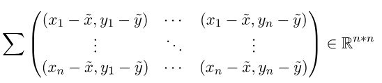
協方差與方差的差別在於，一個是計算本身，一個是計算兩者差異，而協方差公式為向量X和Y每個x和y扣掉各自平均的平方，如下圖。

看公式能得知方差是計算自己的離散程度，而協方差則是計算兩個向量的離散程度(相似性)。

協方差矩陣

將協方差公式輸入帶入垂直行向量與水平列向量，兩者扣除平均相乘則會變為矩陣相乘。公式(E代表平均)帶入為。接著以下舉個較明瞭的實例。

假設，


帶入cov公式，

可看到所產生的結果為R^n*n大小(R為線性代數的向量次方則是維度)，更明瞭來說就是計算X向量的每一個元素與Y向量每一個元素的差距，最後總和即是差異值。

格拉姆矩陣

在影像風格處理當中，風格損失函數使用格拉姆矩陣來計算目前的損失量，而格拉姆矩陣與協方差矩陣類似，差別在於格拉姆矩陣無扣掉均值。它所使用公式為，，從公式可以得知格拉姆矩陣是在計算每個元素和每個元素之間的影響大小的總和。

這時你可能會疑惑為何不用原始影像做處理，主要因為原始影像是包含了顏色、紋理和位置等等特徵(所以主要影像的損失會用原始影像計算)，而格拉姆矩陣則單純計算元素與元素的影響，所以位置不一定要在原來位置也能計算出相同結果，然而結果就會變為新風格加入主要影像。

以下為X矩陣大小1*N的格拉姆矩陣公式，由公式能得知它所產生出來的是一個對稱的三角矩陣，而三角矩陣特性在計算特徵值時候是非常快速的，三角矩陣還有其他特性但這裡沒使用到先暫時略過。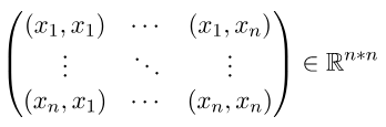

影像風格轉換

影像風格依照[2]輸入影像所使用層為['relu4_1']，風格輸入影像所使用層數為['relu1_1', 'relu2_1', 'relu3_1', 'relu4_1', 'relu5_1']，公式依照[4]所發表的公式實作。

損失公式

主要影像損失函數

使用均方誤差函數，目前輸入資料與主要影像輸入比較。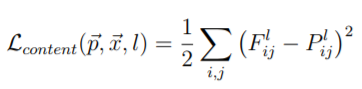

• content_feature為原始影像權重。
• vgg_layer為目前訓練的權重。

def content_loss(content_feature, vgg_layer):
    return tf.nn.l2_loss(vgg_layer - content_feature)

格拉姆矩陣

轉置矩陣乘上原始矩陣。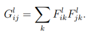

風格影像損失函數

將計算後的格拉姆矩陣使用均方誤差函數，目前輸入資料與主要影像輸入比較。而作者在這裡定義的損失函數的除法MN是要計算使用格拉姆矩陣後的平均，1/4則是方便微分。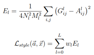

• style_feature為風格影像權重的格拉姆矩陣。
• vgg_layer為目前訓練的權重。
• vgg_feats為展開成二維陣列。
• vgg_gram為計算格拉姆矩陣。

def style_loss(style_feature, vgg_layer):
    K, height, width, channel = map(lambda i: i.value, vgg_layer.get_shape())
    vgg_feats = tf.reshape(vgg_layer, (-1, channel))
    vgg_gram = tf.matmul(tf.transpose(vgg_feats), vgg_feats)

    #M = K * height * width, N = channel
    loss_base = ((K * height * width) ** 2) * (channel ** 2) * 2
    return tf.nn.l2_loss(vgg_gram - style_feature) / loss_base

總損失函數

將主要影像損失函數加上風格影像損失函數即是總損失函數。跑迴圈計算每一層的損失函數並加總。

• content_feature為原始影像權重。
• style_feature為風格影像權重的格拉姆矩陣。
• vgg_layer為目前訓練的權重。

def loss(content_features, style_features, vgg_layers):
    content_loss_total = 0.0
    for name in CONTENT_LAYERS:
        content_loss_total += content_loss(content_features[name], vgg_layers[name])

    style_loss_total = 0.0
    for index in range(len(STYLE_PATH)):
        for name in STYLE_LAYERS:
            style_loss_total += style_loss(style_features[index][name], vgg_layers[name])
    
    style_loss_total /= len(STYLE_LAYERS)
    loss_total = CONTENT_WEIGHT * content_loss_total + STYLE_WEIGHT * style_loss_total
    return loss_total

訓練

初始化參數

• CONTENT_WEIGHT內容影像權重。
• STYLE_WEIGHT風格影像權重。
• CONTENT_LAYERS內容影像特徵網路層。
• STYLE_LAYERS風格影像特徵網路層。
• LEARNING_RATE訓練率。
• TRAIN_TIMES訓練次數。

CONTENT_WEIGHT = 7.0
STYLE_WEIGHT = 400.0
CONTENT_LAYERS = ['relu4_1']
STYLE_LAYERS = ['relu1_1', 'relu2_1', 'relu3_1', 'relu4_1', 'relu5_1']
LEARNING_RATE = 10.0
TRAIN_TIMES = 1000

影像存取函數

論文使用白化處理，這裡偷懶一點直接扣除一半的像素。

def imsave(path, img):
    img = np.clip(img + 128, 0, 255).astype(np.uint8)
    scipy.misc.imsave(path, img)

def imread(path):
    return scipy.misc.imread(path).astype(np.float) - 128

初始化原始特徵網路

1. content_image讀取後扣掉RGB均值或VGG預設均值(扣128)。
2. content_image轉為四維。
3. 計算CONTENT_LAYERS層內的權重。
   style_image也是相同只是多計算格拉姆。

# init
content_features = {}
style_features = [{} for _ in STYLE_PATH]

with tf.Session() as session:
    content_image = imread(CONTENT_PATH)
    #content_mean = np.mean(np.mean(content_image, axis=0), axis=0)
    #content_image -= content_mean
    content_4d_shape = (1,) + content_image.shape
    content_image = np.reshape(content_image, content_4d_shape)
    vgg_input = tf.placeholder(tf.float32, shape=content_4d_shape)
    nets = vgg19.VGG19_build(VGG_PATH, vgg_input)
    for name in CONTENT_LAYERS:
        content_features[name] = session.run(nets[name], feed_dict={vgg_input: content_image})

with tf.Session() as session:
    for index in range(len(STYLE_PATH)):
        style_image = imread(STYLE_PATH[index])
        #style_mean = np.mean(np.mean(style_image, axis=0), axis=0)
        #style_image -= style_mean
        style_4d_shape = (1,) + style_image.shape
        style_image = np.reshape(style_image, style_4d_shape)
        vgg_input = tf.placeholder(tf.float32, shape=style_4d_shape)
        nets = vgg19.VGG19_build(VGG_PATH, vgg_input)
        for name in STYLE_LAYERS:
            style_feature = session.run(nets[name], feed_dict={vgg_input: style_image})
            style_feats = np.reshape(style_feature, (-1, style_feature.shape[3]))
            style_gram = np.matmul(style_feats.T, style_feats)
            style_features[index][name] = style_gram

訓練

1. initial為隨機初始化影像權重，並存入Tensor型態的image。
2. nets為初始化要訓練的神經網路。
3. loss_op為計算目前損失。
4. train_op為使用Adam訓練。
5. 訓練至TRAIN_TIMES次即可。

initial = None
with tf.Graph().as_default():
    if initial is None:
        initial = tf.random_normal(content_4d_shape) * 1
    else:
        initial = np.array([initial])
        initial = initial.astype('float32')

    image = tf.Variable(initial)
    nets = vgg19.VGG19_build(VGG_PATH, image)

    loss_op = loss(content_features, style_features, nets)

    train_op = tf.train.AdamOptimizer(LEARNING_RATE).minimize(loss_op)

    min_loss = 10000000000000
    with tf.Session() as session:
        session.run(tf.global_variables_initializer())
        for time in range(TRAIN_TIMES):
            train_op.run()
            now_loss = loss_op.eval()
            print(time, ":", now_loss)
            if now_loss < min_loss:
                min_loss = now_loss
                save_image = image.eval()
                imsave('Image/' + str(time) + '.jpg', save_image[0])
        imsave('Image/final.jpg', save_image[0])

結果

內容影像。

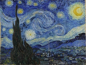
風格影像。

結果。

結語

在[2]中有修改一些公式，訓練出來的資料也不錯，這也代表損失函數可以加入自己的公式和想法，並創造出不同的風格，其實延伸至其他網路也是如此，但要做出屬於真正可用的公式我想要有一定的數學知識，否則也很難達到真正所需的效果。

參考網址與書籍

[1] https://www.tensorflow.org/api_docs/python/tf
[2] 籃子軒(譯者)（2018）。Deep Learning深度學習基礎｜設計下一代人工智慧演算法。台灣：歐萊禮。
[3]Karen Simonyan, Andrew Zisserman,"Very Deep Convolutional Networks for Large-Scale Image Recognition".arXiv:1409.1556, 2015
[4]Leon A. Gatys, Alexander S. Ecker, Matthias Bethge,"A Neural Algorithm of Artistic Style".arXiv:1508.06576, 2015
[5] https://zhuanlan.zhihu.com/p/37609917
[6] https://upmath.me/