簡單回顧
在前幾章，我們從什麼是機器學習，機器學習的架構（given dataset D -> find H -> get g），及了解什麼是classification。這個章節會介紹什麼是Perceptron Learning Algorithm（PLA），並且實作binary classification。

Perceptron
以銀行發放信用卡為例，由下面圖中可以得知，xi代表的是客戶的資特徵值，也就是會對結果造成影響的參數，在這裡指的是age、annual salary…，但是每個特徵值對結果影響的比重都不一樣，可能annual salary比age影響來的大，所以給它的wi也比較大，這個wi我們稱為權重(weight)。

在計算完所有的特徵值之後，算出來的值必須超過某個門檻值，銀行才能決定是否發放信用卡給客戶（就像在學校考試，有作業成績，期中考，期末考，可能期中期末的比重較重，那教授要不要把你當掉，當然就是看學期平均是否有高過門檻值囉）這個門檻值就是threshold。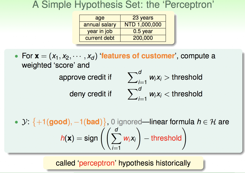

其實theshold也可以看成是線性組合的一部分，如下圖所示，可以把theshold也做合併，式子看起來比較簡短。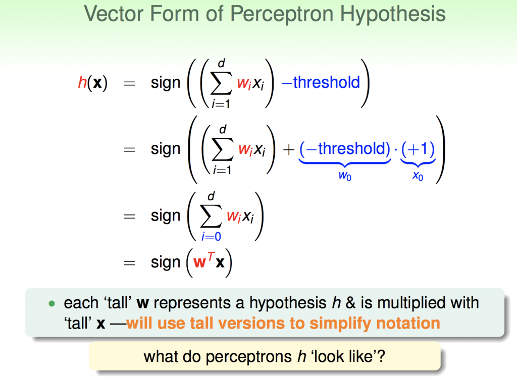

我們可以把這個抽象的數學式子變成具體的圖像，在這邊我們可以把資料代入h(x)，如果結果>0就以藍色o表示；反之，<0就以紅色x表示，在這個二維平面上存在許多h(x)，而每一個h(x)都能形成一條直線來分類資料，如果能找到一個h(x)，能完美的分割所有資料，這就是所謂的分類，而Perceptrons就是一種線性分類器。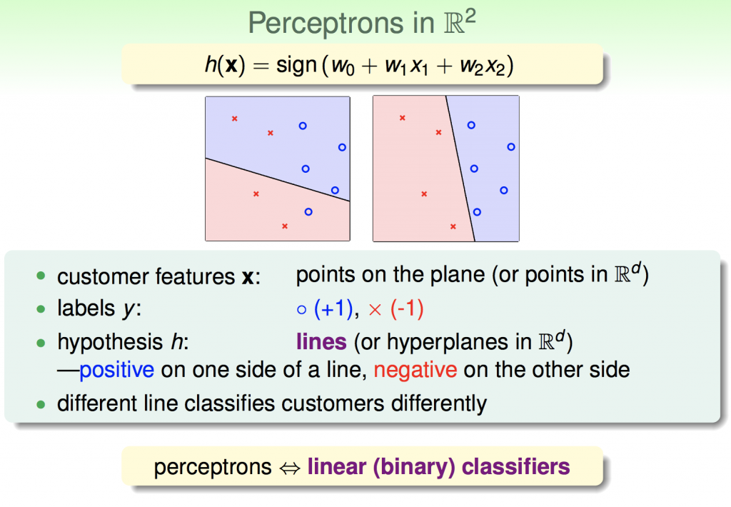

Perceptron Learning Algorithm
在這個二維平面上存在無限多條直線，那要如何選擇一條線可以完美分類我們的資料？最簡單的做法就是，先隨機選擇一條直線（假設h=w0 * x），然後不段的修正它，直到這條直線可我完整地分類所有資料。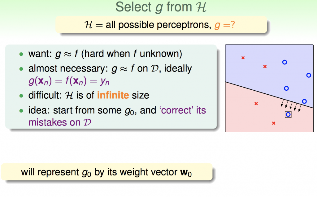

下面這張圖告訴我們如何對錯誤做修正，假設今天有一個點分類錯誤，實際上我們提供的資料結果是要核發信用卡，但是分類結果卻是不核發信用卡，也就是我們實際上x結果與w出來結果的夾角太大，我們可以透過向量加減來修正它，直到不再犯錯為止（圖片中t代表第幾次修正）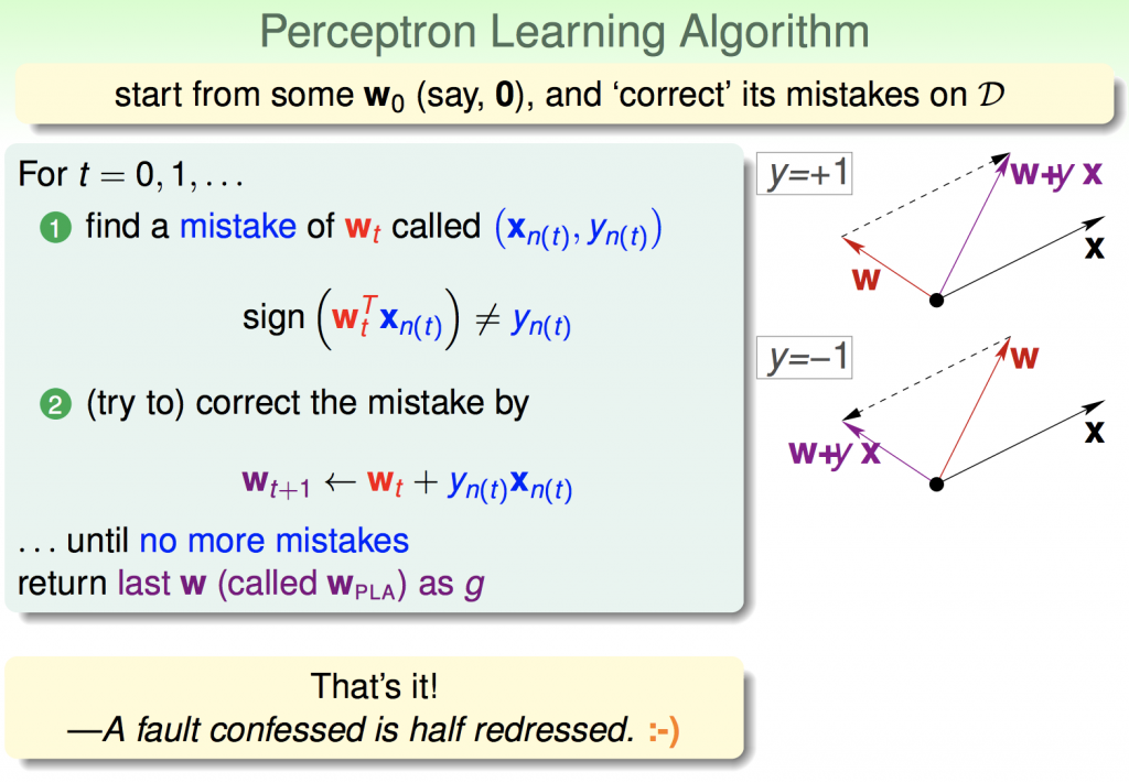

鳶尾花數據實作感知器模型

import numpy as np
import pandas as pd
import matplotlib.pyplot as plt


class Perceptron:
    def __init__(self, eta=0.01, n_iter=10):
        self.eta = eta
        self.n_iter = n_iter

    def fit(self, X, y):
        self.w = np.zeros(1 + X.shape[1])
        self.errors = []

        for _ in range(self.n_iter):
            error = 0
            for xi, target in zip(X, y):
                update = self.eta * (target - self.predict(xi))
                self.w[1:] += update * xi
                self.w[0] += update
                error += int(update != 0.0)
            self.errors.append(error)
        return self

    def net_input(self, X):
        return np.dot(X, self.w[1:]) + self.w[0]

    def predict(self, X):
        return np.where(self.net_input(X) >= 0.0, 1, -1)
  

def main():
    df = pd.read_csv('https://archive.ics.uci.edu/ml/machine-learning-databases/iris/iris.data', header=None)
    X = df.iloc[0:100, [0, 2]].values
    y = df.iloc[0:100, 4].values
    y = np.where(y == 'Iris-setosa', -1, 1)
    
    plt.scatter(X[:50, 0], X[:50, 1], color='red', marker='o', label='setosa')
    plt.scatter(
        X[50:100, 0],
        X[50:100, 1],
        color='blue',
        marker='x',
        label='versicolor')
    plt.xlabel('petal length')
    plt.ylabel('sepal length')
    plt.legend(loc='upper left')
    plt.show()

if __name__ == '__main__':
  main()