3. Variable transformation

一些機器學習模型，例如線性回歸(linear regression) 或 logistic regression 都假設變數下的資料是常態分布(normal distribution 或稱高斯分布 Gaussian)；而其他的學習模型也可從變數資料常態分布獲益，因為在常態分布下，變數值跨越的更大的範圍，而這些變數是用來預測Y值(label or target)的，因此，可能會提高機器學習演算法的表現。

假如變數不是常態分布，我們可以使用數學公式，將變數下的資料轉換為常態分布。下列是可使用的數學公式，至於要選擇哪個端視原始資料的分布。

3.1 Logarithm transformation - log(x)
3.2 Reciprocal transformation - 1 / x
3.3 Square root transformation - sqrt(x)
3.4 Exponential transformation - exp(x)
3.5 Yeo-Johnson transformation
3.6 Box-Cox transformation

以 Kaggle 的 Titanic 資料集中的"年齡"變數來說明：

import pandas as pd
import numpy as np
import matplotlib.pyplot as plt
%matplotlib inline
import pylab
import scipy.stats as stats

train_data = pd.read_csv('../input/titanic/train.csv', usecols=['Age', 'Fare','Survived'])
train_data.head()

Rec-no| Survived| Age| Fare
------------- | -------------
0 | 0| 22.0 | 7.2500
1 | 1 | 38.0 | 71.2833
2 | 1 | 26.0| 7.9250
3 | 1| 35.0 | 53.1000
4 | 0| 35.0 | 8.0500
.. | ...| ...| ...
886| 0 | 27.0| 13.0000
887| 1 | 19.0| 30.0000
888 | 0| NaN| 23.4500
889| 1| 26.0| 30.0000
890| 0| 32.0| 7.7500

把缺年齡的位置補齊，缺額共177筆，從現有年齡資料中隨機挑選177筆數值補上。

def impute_na(data, variable):
    # fill na with a random sample
    df = data.copy()
    
    # random sampling
    df[variable+'_random'] = df[variable]
    
    # extract the random sample to fill the na
    random_sample = df[variable].dropna().sample(df[variable].isnull().sum(), random_state=0)
    
    random_sample.index = df[df[variable].isnull()].index
    df.loc[df[variable].isnull(), variable+'_random'] = random_sample
    
    return df[variable+'_random']
    
train_data['Age'] = impute_na(train_data, 'Age')

以長條圖和QQ圖(Q-Qplot)來檢視資料，如果資料點都集中在QQ圖的直線上，我們可推論這是常態分布。

def diagnostic_plots(df, variable):
    plt.figure(figsize=(15, 6))
    plt.subplot(1, 2, 1)
    df[variable].hist()
    
    plt.subplot(1,2, 2)
    stats.probplot(df[variable], dist="norm", plot=pylab)
    plt.show()
    
diagnostic_plots(train_data, 'Age')  

3.1 Logarithm transformation - log(x)

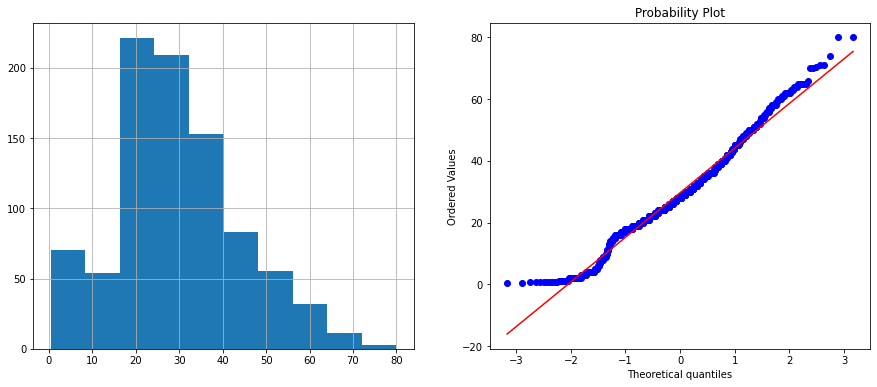
這是最常見的方法。

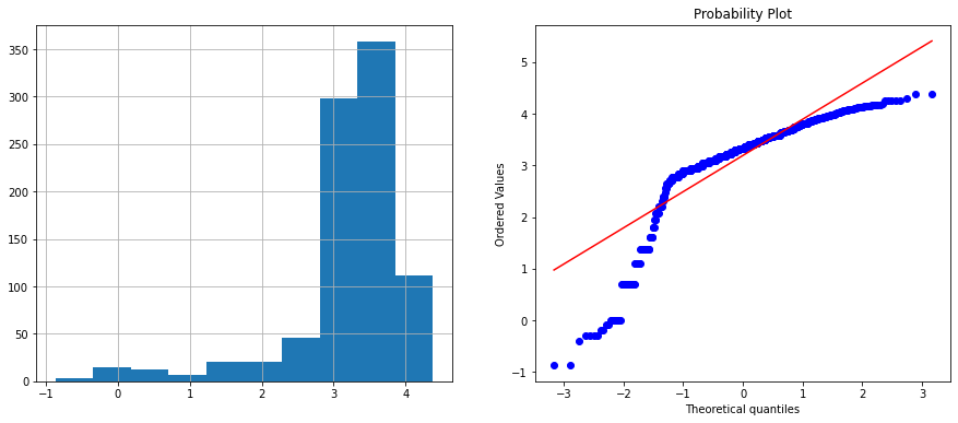
train_data['Age_log'] = np.log(train_data.Age)
diagnostic_plots(train_data, 'Age_log')

3.2 Reciprocal transformation - 1 / x

train_data['Age_reciprocal'] = 1 / train_data.Age
diagnostic_plots(train_data, 'Age_log')

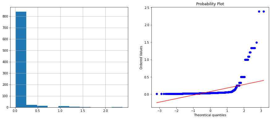
和第一個方法一樣轉換後的結果並不理想。

3.3 Square root transformation - sqrt(x)

train_data['Age_sqr'] = train_data.Age**(1/2)
diagnostic_plots(train_data, 'Age_sqr')

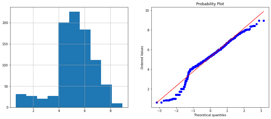
和前面兩個比起來，效果比較好，然而它還不是常態分佈，而和原始資料比起來改善不大。