
前面提到了訓練一個 Neural Network 包含 prediction 和 training 兩大步。這篇會深入介紹一下 training 這一步。
本篇數學偏難,但實際應用並不需要完全理解,所以不需擔心看不懂喔。這邊撐過去後面好玩多了!
在取得 prediction 之後,我們會計算這個預測值跟實際答案的誤差,並反向回饋給 network 裡的 parameters。後面這步也稱 backpropagation。訓練步驟大致如下:
Loss function 決定這個 network 是怎麼衡量誤差的,因此會根據資料屬性不同選擇不同的 loss function。
我們通常用 代表 prediction,y 代表 label。以下介紹兩種常見 loss function 和應用場合:
| Mean Squared Error (MSE) | Cross-Entropy Loss | |
|---|---|---|
| Function | ||
| 應用場合 | Regression | Multiclass classification |
注意式子都是針對單一 data sample。
MSE 適用預測一個數值的 regression ,因此 y 和 都是 scalar value(純量)。
Cross-Entropy 則適用預測種類的 multiclass classification,前篇有提到在做 multiclass classification 最後 output 會是 C 個機率值(C 為種類數),所以這裡 y 和 是大小為 C 的 vector,
和
則是 vector 的第 i 個值。而 cross-entropy loss 就是每個種類計算
並加總。
這邊注意的是 y 其實是 one-hot vector,也就是整個 vector 只有一個位置是 1 其餘為 0,而 1 就在正確種類的位置。所以說雖然在做加總,實際上只會有一個 ,所以式子可以簡化為
,c 為正確種類的位置。是不是簡單很多?
在 multiclass classification 有時候 y 也可以是 scalar value,代表正確種類的位置。不管是數學式子還是寫 code 時用到的 loss function,都應該依照前後文判斷 y 是 scalar 還是 vector。
對 Cross-Entropy 這個式子感到恐懼的我理解你,這是在 information theory 裡衡量兩個機率分佈有多不一樣的一個方法,deep learning 新手就使用就好,阿密陀佛。
要來到重頭戲了。切記先複習一下 matrix differentiation(矩陣微分),以及 partial differentiation(偏微分)的概念。
這邊有很多數學,所以先來張圖比較好講解:

—— Two hidden layer network for binary classification。[1]
這邊我們用 來表示第
層,(i) 來表示第 i 筆資料。
、
、
、
都參照前篇介紹的表示法。
好,我們在右端計算了 loss L,現在要從右到左告知 network 裡的所有 parameters 他們做得有多差,請他們修正自己以減少下次的 loss。
那要怎麼知道需要往哪裡修正多少?這就跟 Gradient Descent(梯度下降法) 有關了。

—— Sample loss function visualization。[2]
先來視覺化一下 loss function。圖中 是一個 vector,
為第 i 個 parameter,這個簡單的 model (跟前面圖的 model 不同)總共有兩個 parameter,而
是 loss 值。
目前我們 model 的 parameter 在紅點點那邊,造成的 loss 很高,可以說是表現很差。而綠點點是 model 能得到最好的表現,因為誤差最小。我們希望可以讓 parameter 的值往綠點點的方向移動。
這聽起來很簡單。但在現實世界裡,parameters 可不只兩個,維度一高圖形可就沒那麼簡單,要知道綠點的準確位置一點都不實際。但有個辦法:就往低處走吧?水往低處流,雖然不一定會走在捷徑上,總有一天也會到谷底。
也就是找出橘色的向量。仔細一看,他好像是⋯⋯紅點在曲面上的切線?
還記得怎麼在二維平面找出一條切線的斜率嗎?沒錯,取 derivative 。那麼在高維空間找切線呢?那肯定就是取 gradient 了。
Gradient 可以說是多維度的 derivative,基本上就是幫 vector 裡的所有值取 partial derivative。以這張圖為例,對 parameters 取 gradient 為:

Partial derivative (偏微分)很簡單啦,就是針對一個維度取微分。方法跟微分一樣,但把其他維度的值當成常數即可。
所謂 descent 就是下降,所以 gradient descent 就是找出並沿著切線,一路盲目往低處走,以尋找最佳解。
介紹完 gradient descent,回到原本的 model,我們是要讓 parameters 知道自己要往哪個方向修正對吧。沒錯,就是計算 L 對 的 gradient。
因為是做分類問題,我們用 cross-entropy 當作 loss function:

這裡因為是 binary classification,y 是 scalar value 1 或 0。
所以有以下 6 組 gradient 要算:

相信到這邊大家一定腦袋空白。好前面我都懂,但課本讀完讀題目怎麼像之前什麼都沒讀過?完全沒有頭緒。
總之,我們先從最後一層看起。我們會看到如果一層一層往前算,搭配微積分裡的 Chain Rule,計算方法會簡化許多。
先複習一下 chain rule。他是用來取 composite function f(g(x)) 的微分的:
where z = g(x)。

我們先看一下最後一層, 是怎麼計算出來的:

這邊因為是 binary classification,g 為 sigmoid function。
這一層有兩組 parameters: 和
。我們示範
就好。如果要硬幹他的 gradient 的話,結合前幾個式子,可以得到:
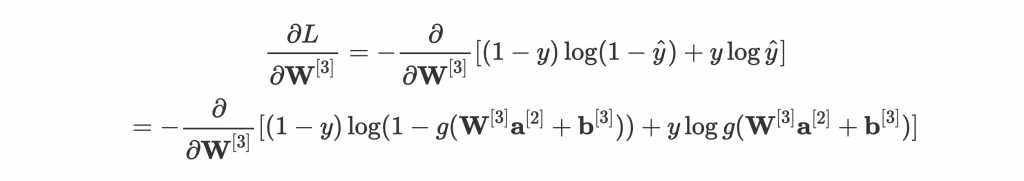
喂等等先不要離開啊!我們沒有要嘗試化簡這個式子的意思。雖然現在上下有 可以開始手算,但實在太複雜,而且對 engineering 來說也很不實際。總不會寫一個 network 就要把這些式子爆開 code 進去吧?
這時候我們應用 chain rule,優雅的簡化成三步驟:
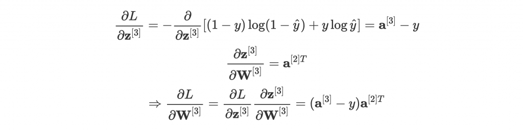
不只數學計算簡單多了,在寫程式的時候,也可以把這些步驟分開來,並針對不同 loss 或 activation function 寫 gradient,分別計算後乘在一起就行。
詳細數學推導請見 [1] p.11-12,或自己練習。
是怎麼來的?
首先
,因為取偏微分所以
當常數微掉變 0,
也可以想像成
對 x 微分剩 c,所以剩
。
那為什麼要取 transpose 呢?因為對 matrix A 微分的結果必然是 A 的形狀。
的形狀是
,
,所以要取 transpose 才符合
蛤你又問為什麼知道
第二層有兩個 node 所以
。最後
的結果取決於第三層有幾個 node 所以是
自然是
更直觀的看法就是
會是
,
代表第 i 層有幾個 node。
好了小秘訣都說完了,不可以再抱怨太複雜因為很多資料連小秘訣都沒有。

運用 chain rule,先把 forward propagation 的式子列出來,再由後往前找出對中間值的 gradient,就能依樣畫葫蘆找出其他 和
了。
也因為要先從後面的 layer 開始計算,並把結果往前送,這個過程才被稱為 backpropagation。
那就試著自己找出前面幾個 parameter 的 gradient 吧。還是不熟悉的可以參考 [1] p.11-12!
上面取 gradient 的部分應該是全系列最數學的地方,我也盡量提供一些訣竅幫助理解。如果反覆看幾次還是如在霧裡,那我跟你說沒關係,應用方面需要理解的數學不會這麼深!
好的,那還記得我們取 gradient 是尬麻嗎?是要找出往低處走的方向。找出來以後,我們要實際讓這些 parameters 邁出步伐,修正自己。
修正的方式很簡單:

這邊我們統稱 parameters 為 ,就是
和
啦。
我們知道剛剛讓人困擾終於搞懂的 是我們要前進的方向,那
就是步伐大小了。我們稱之為 learning rate,也就是學習速率。減號是因為是要減小 L 的值,所以是走 L 的負方向。用此方式 update,parameters 就會往低處前進了。
那老師,為什麼不就走很大步就好呢?這樣不就學很快?
我們來看看這張圖:
—— Learning rate 影響學習成果。[4]
Learning rate 太低的話,training 會很慢;但太高的話,又容易走過頭。因此選擇適當的 learning rate 其實是一門藝術!後面也會講到怎麼依據學習情況自動調節 learning rate。
請問接著要怎麼利用chain rule微分阿?
還是可以列出leve 2的偏微分是長什麼樣子嗎?
唉原來參考資料有推導 
我懂了,平常剝洋蔥要用這個
Fs_n( a[n-1] ) = W[n]a[n-1]+b[n] = z[n]
但遇到W[target]時要換用這個
Fs_n( W[n] ) = W[n]a[n-1]+b[n] = z[n]
遇到b[target]時要換用這個
Fs_n( b[n] ) = W[n]a[n-1]+b[n] = z[n]
上面第1張圖可以轉換成這樣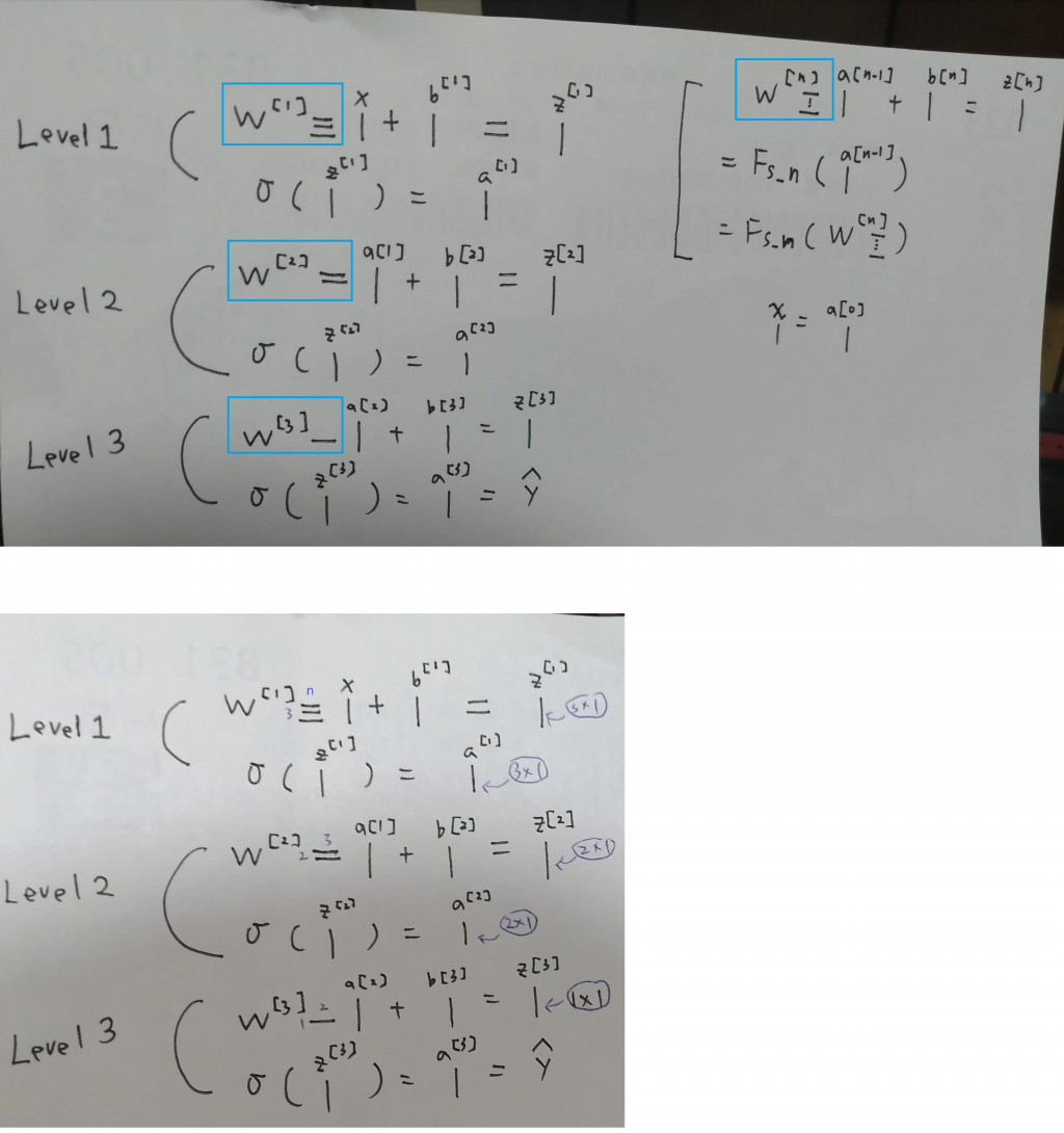
寫成這樣好了,其實不用拆3種呢
Fs_n( W[n],a[n-1],b[n] ) = W[n]a[n-1]+b[n] = z[n]
//////////////
P12頁最後的結果是|2x3|矩陣
但它推導過程標註的陣列大小是不是有點怪怪的阿?
。這個符號上面說是Hadamard produc
google後看起來比較像是The penetrating face product
那4組導數相乘,看起來過程要這樣
|1x1||1X2|。|2X2||2X3|
=|1X2|。|2X2||2X3|
=|2X2||2X3|
=|2X3|
不是才會得到|2X3|矩陣嗎?
然後照著它的思路推進到 ∂ L / ∂ W[1] 時
會有6組導數相乘,而且最後的結果是|3Xn|矩陣
如果我寫成
|1x1||1X2|。|2X2||2X3|。|3X3||3Xn|
=|2X3|。|3X3||3Xn|
|2X3|。|3Xn|要怎麼做The penetrating face product?
如果拿掉第1個。寫成
|1x1||1X2||2X2||2X3|。|3X3||3Xn|
=|1X2||2X2||2X3|。|3X3||3Xn|
=|1X2||2X3|。|3X3||3Xn|
=|1X3|。|3X3||3Xn|
=|3X3||3Xn|
=|3Xn|
就可以得到|3Xn|矩陣也
但真的是這樣做的嗎?
//////////////
我又比較了一下
|1X2|。|2X2|和|1X2||2X2|
|1X2|。|2X2| = |A B|。|a 0| = |Aa 0|
                      |0 b|   |0 Bb|

|1X2||2X2| = |Aa Bb|
2者挾帶的資訊量其實是一樣的
差別是,遇到接下來的陣列|2X3|
一個會分配
|1X2|。|2X2||2X3|
|Aa 0| |x y z| = Aa|x y z|
|0 Bb| |u v w|   Bb|u v w|
一個會合併
|1X2||2X2||2X3|
|Aa Bb||x y z| = Aa|x y z| + Bb|u v w|
       |u v w|


