只有距離。
有 distance 距離與 direction 方向。
超過三維以上則稱 tensor 張量
以下會主要以向量為主討論。
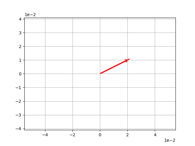
import numpy as np
import matplotlib.pyplot as plt

# We'll use a numpy array for our vector
v = np.array([2,1])
origin = [0], [0]

plt.axis('equal')
plt.grid()
plt.ticklabel_format(style='sci', axis='both', scilimits=(0,0))
plt.quiver(*origin, *v, scale=10, color='r')    # quiver畫箭頭,*表示展開

plt.show()
import numpy as np

vMag = np.linalg.norm(v)
print (vMag)

>>  2.23606797749979
例子:tan(a) = 1/2,則 a = tan−1(0.5) ≈ 26.57
import math
import numpy as np

# 向量座標
v = np.array([2,1])
vTan = v[1] / v[0]
print ('tan = ' + str(vTan))

>>  tan = 0.5

# 三角函數轉換
vAtan = math.atan(vTan)
print('radian =', vAtan)                   # 逕度

>>  radian= 0.4636476090008061

# 或 math.degrees(vAtan)
print('degree =', vAtan*(360/(2*math.pi))) # 角度

>>  degree = 26.56505117707799
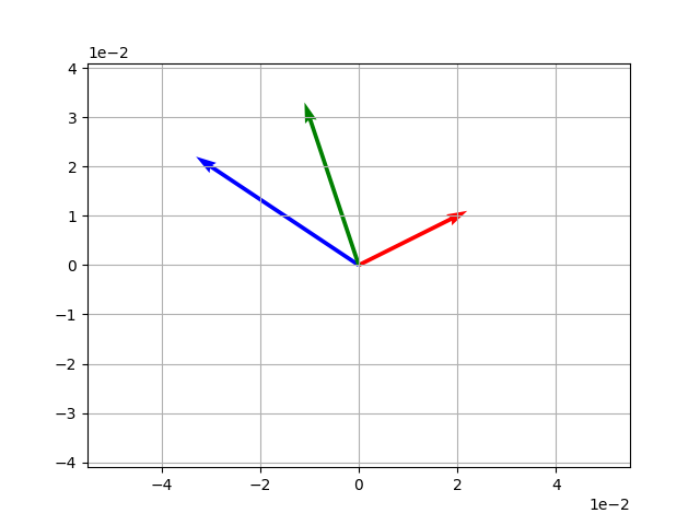
# 1-4. Vector add
import math
import numpy as np
import matplotlib.pyplot as plt

v = np.array([2, 1])    # 力 1
s = np.array([-3, 2])   # 力 2
z = v + s               # 合力

# Plot v and s
vecs = np.array([v, s, z])
origin = [0, 0, 0], [0, 0, 0]
plt.axis('equal')
plt.grid()
plt.ticklabel_format(style='sci', axis='both', scilimits=(0,0))
plt.quiver(*origin, vecs[:, 0], vecs[:, 1], color=['r', 'b', 'g'], scale=10)

plt.show()
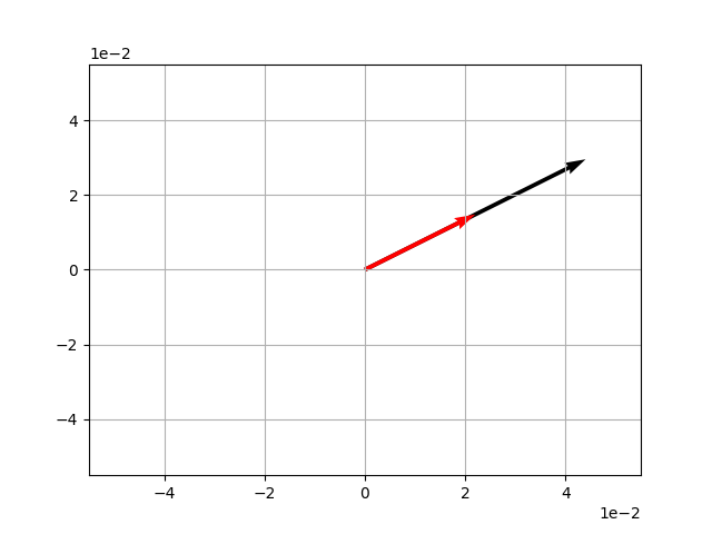
import numpy as np
import matplotlib.pyplot as plt
import math

v = np.array([2,1])
w = 2*v

# 作圖
vecs = np.array([w, v])
origin = [0, 0], [0, 0]
plt.grid()
plt.ticklabel_format(style='sci', axis='both', scilimits=(0,0))
plt.quiver(*origin, vecs[:, 0], vecs[:, 1], color = ['k', 'r'], scale=10)

plt.show()
vs = (v1s1) + (v2s2) + ... + (vnsn)
數學意義為 v 在 s 上的投影,物理意義為對特定方向"作功"。
數學證明如下: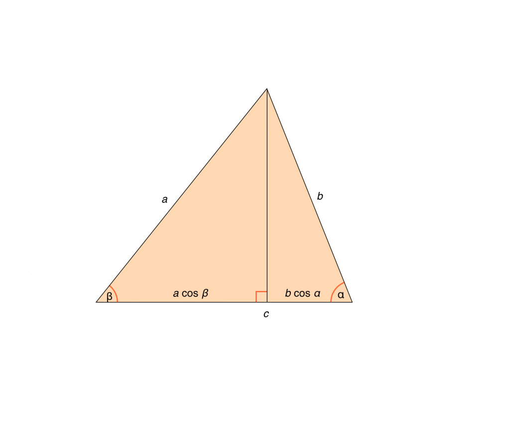
import numpy as np

v = np.array([2, 1])
s = np.array([-3, 2])

d = v @ s
# 或 d = v.dot(s)
print(d)

>>  -4
當然,換個說法
以下是 python 的實際程式碼:
import math

vMag = np.linalg.norm(v)
sMag = np.linalg.norm(s)

cos = v @ s / (vMag * sMag)
theta = math.degrees(np.arccos(cos))

print(theta)

>>  119.74488129694222
import numpy as np

X = np.arange(1,7).reshape(2,-1)  # -1 會自動計算合理的分配數
print(X)

>>  [[1 2 3]
    [4 5 6]]
首先,我們建立三個矩陣:
import numpy as np
A = np.array([[1,2,3],
              [4,5,6]])
B = np.array([[6,5,4],
              [3,2,1]])
C = np.array([[9,8],
              [7,6],
              [5,4]])
print(A + B)

>>  [[7 7 7]
    [7 7 7]]
print(A - B)

>>  [[-5 -3 -1]
    [ 1  3  5]]
C1. Scalar Multiplication
print(2 * A)

>>  [[ 2  4  6]
    [ 8 10 12]]
C2. Dot
print(A @ C) # 矩陣 2*3 x 矩陣 3*2 → 矩陣 2*2

>>  [[ 38  32]
    [101  86]]

print(C @ A) # 矩陣 3*2 x 矩陣 2*3 → 矩陣 3*3

>>  [[41 58 75]
    [31 44 57]
    [21 30 39]]
不論任何矩陣乘以單位矩陣,都將等於自身矩陣。
import numpy as np
A = np.array([[1,2,3],
              [4,5,6],
              [7,8,9]])
one = np.eye(3)
print(one)

>>  [[1. 0. 0.]
    [0. 1. 0.]
    [0. 0. 1.]]

print(A @ one)

>>  [[1. 2. 3.]
    [4. 5. 6.]
    [7. 8. 9.]]
任何矩陣乘以自身反矩陣會等於單位矩陣。
A.A^-1 = I
import numpy as np
a = np.array([[1, 2],
              [3, 4]
             ])
print(np.linalg.inv(a))

>>  [[-2.   1. ]
    [ 1.5 -0.5]]
x + y = 16
10x + 25y = 250
提示:A.X = B,則 X = A^−1.B
A = np.array([
    [1, 1],
    [10, 25]])
B = np.array([16, 250])
print(np.linalg.inv(A) @ B)
# 其結果會等同 np.linalg.solve(A, B)

>>  [10.  6.]
常在特徵轉換(降維)的過程中用到,以下分開解釋。
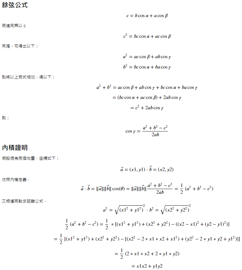
import numpy as np
import matplotlib.pyplot as plt

v = np.array([1, 0])
A = np.array([[2,1],
              [1,2]])

t = A @ v

original = [0], [0]
plt.axis('equal')
plt.grid()
plt.ticklabel_format(style='sci', axis='both', scilimits=(0, 0))
plt.quiver(*origin, *t, color='orange', scale=10)
plt.quiver(*origin, *v, color='blue', scale=10)
plt.show()
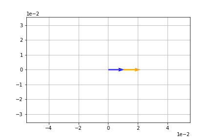
import numpy as np
import matplotlib.pyplot as plt

v = np.array([1,0])
A = np.array([[0,-1],
              [1,0]])

t = A@v
print (t)

origin = [0], [0]
plt.axis('equal')
plt.grid()
plt.ticklabel_format(style='sci', axis='both', scilimits=(0,0))
plt.quiver(*origin, *t, color='orange', scale=10)
plt.quiver(*origin, *v, color='blue', scale=10)

plt.show()
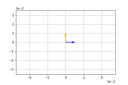
import numpy as np
import matplotlib.pyplot as plt

v = np.array([1,0])
A = np.array([[2,1],
              [1,2]])

t = A@v
print (t)

origin = [0], [0]
plt.axis('equal')
plt.grid()
plt.ticklabel_format(style='sci', axis='both', scilimits=(0,0))
plt.quiver(*origin, *t, color='orange', scale=10)
plt.quiver(*origin, *v, color='blue', scale=10)

plt.show()
當變換僅"影響尺度"時"變換矩陣"與"常數"等效:
v = np.array([1,0])
A = np.array([[2,0],
              [0,2]])

t1 = A@v
t2 = 2*v

print(t1, t2)
>>  [2 0] [2 0]
當然,numpy 很貼心的提供了 Eigenvectors and Eigenvalues 的算法:
import numpy as np
A = np.array([[2, 0],
              [0, 3]])
eVals, eVecs = np.linalg.eig(A)
print('Eigenvalue:\n', eVals)
print('Eigenvector:\n', eVecs)

>>  Eigenvalue:
     [2. 3.]
    Eigenvector:
     [[1. 0.]
     [0. 1.]]
.
.
.
.
.
import numpy as np
import matplotlib.pyplot as plt
from sympy.core.symbol import Symbol

# 梯度下降法
def GD(x_start, df, epochs, lr):
    xs = np.zeros(epochs+1)
    x = x_start
    xs[0] = x
    for i in range(epochs):
        dx = df(x)
        x += -dx * lr
        xs[i+1] = x
    return xs
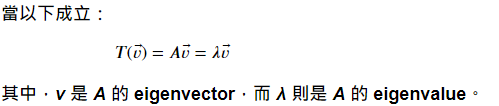
f(x) = x^3 - 2x + 100
超參數:
x_start = 2
epochs = 1000
learning_rate = 0.01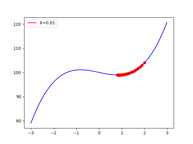
f(x) = -5x^2 + 3x + 6
x_start = 2
epochs = 1000
learning_rate = 0.01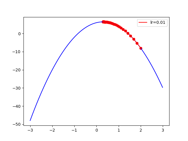
f(x) = 2x^4 - 3x^2 + 2x - 20
x_start = 5
epochs = 1000
learning_rate = 0.001 # 必須要設定小,否則會左右橫跳
f(x) = sin(x)e^(-0.1(x-0.6)^2)
此時要注意先把函數的一階導函數求出來,我們運用 sympy 達成。
from sympy import *
x = Symbol('x')
y = sin(x)* E ** (-0.1*(x-0.6)**2)
dy = y.diff(x) # 把方程式微分求一階導函數

def func(x):
    return np.sin(x)*np.exp(-0.1*(x-0.6)**2)
def dfunc(x_self):
    return dy.subs(x, x_self).evalf() # 把 x_self 用 sub 函數迭代入 dy
接著就可以畫出梯度下降啦,要注意的僅剩下起始點的取值了
4-1.
x_start = 0.3
epochs = 1000
learning_rate = 0.01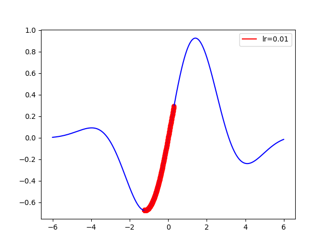
4-2.
x_start = 2.5
epochs = 1000
learning_rate = 0.01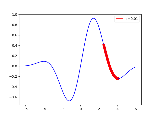
.
.
.
.
.
https://ithelp.ithome.com.tw/articles/10222877?sc=rss.iron
max z = 4x + y
3x + 2y <= 6
6x + 2y <= 10
x, y >=0
對話機器人分析對話,通常會將其轉為矩陣,進行比對才輸出。
#語料
corpus = [
    'This is the first document.',
    'This is the second second document.',
    'And the third one.',
    'Is this the first document?',
    ]
from sklearn.feature_extraction.text import CountVectorizer

#將文件中的詞語轉換為詞頻矩陣
vectorizer = CountVectorizer()

#計算個詞語出現的次數
X = vectorizer.fit_transform(corpus)

#獲取詞袋中所有文件關鍵字
word = vectorizer.get_feature_names()
print ("word vocabulary=", word)
>> word vocabulary= ['and', 'document', 'first', 'is', 'one', 'second', 'the', 'third', 'this']
print ("BOW=", X.toarray())
>> BOW= [[0 1 1 1 0 0 1 0 1]
 [0 1 0 1 0 2 1 0 1]   # 第六個詞 "second" 出現 "2" 次
 [1 0 0 0 1 0 1 1 0]
 [0 1 1 1 0 0 1 0 1]]
from sklearn.feature_extraction.text import TfidfTransformer

transformer = TfidfTransformer()
print ("transformer=", transformer)
>> transformer= TfidfTransformer()

# TF-IDF值
tfidf = transformer.fit_transform(X)

# 查看資料結構 tfidf[i][j] 表示 i 類文件中的 tf-idf 權重
print ("tfidf=", tfidf.toarray())
>> tfidf= [[0.         0.43877674 0.54197657 0.43877674 0.         0.
  0.35872874 0.         0.43877674]
 [0.         0.27230147 0.         0.27230147 0.         0.85322574
  0.22262429 0.         0.27230147]
 [0.55280532 0.         0.         0.         0.55280532 0.
  0.28847675 0.55280532 0.        ]
 [0.         0.43877674 0.54197657 0.43877674 0.         0.
  0.35872874 0.         0.43877674]]
from sklearn.metrics.pairwise import cosine_similarity
print (cosine_similarity(tfidf[-1], tfidf[0:-1], dense_output=False))
>> (0, 2)	0.1034849000930086
  (0, 1)	0.43830038447620107
  (0, 0)	1.0   # 100% 相似 (cos = 1)
 s790502ss

 iThome鐵人賽