Chap.II Machine Learning 機器學習

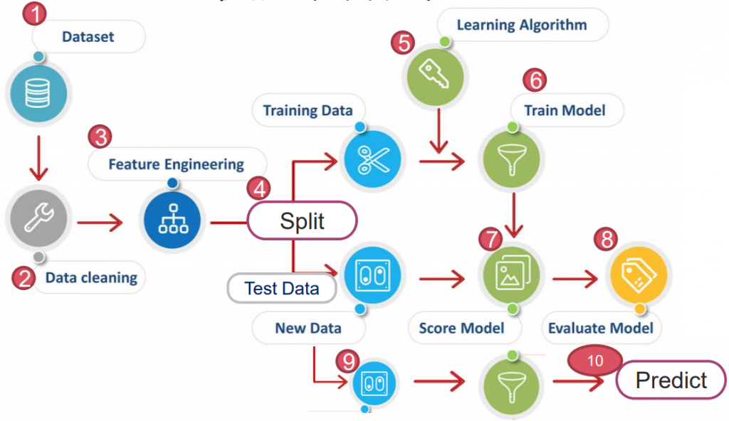
https://yourfreetemplates.com/free-machine-learning-diagram/

Part 4. Evaluation & Performance Tuning 評估與效能調校

4-1. Pipe Line 管線配置

將「縮放」「降維」「演算法」等規劃進管線，方便一次性調校超參數，找出最佳效能。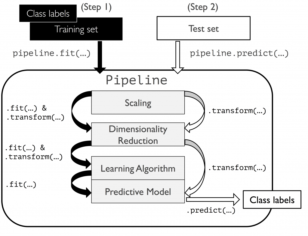

以乳癌為例：

from sklearn.datasets import load_breast_cancer
from sklearn.model_selection import train_test_split

X, y = load_breast_cancer(return_X_y=True)
X_train, X_test, y_train, y_test = train_test_split(X, y, test_size=0.3)

管線化：

from sklearn.pipeline import make_pipeline
from sklearn.preprocessing import StandardScaler
from sklearn.ensemble import RandomForestClassifier as RFC

rfc_PL = make_pipeline(
    StandardScaler(),
    PCA(n_components=2),
    RFC(n_estimators=100, criterion='gini', max_depth=3)
)

rfc_PL.fit(X_train, y_train)
rfc_PL.score(X_test, y_test)

>>  0.9239766081871345

我們使用 make_pipeline 中省去了轉換資料放入標準化、PCA 與演算法等時間。

那麼，知道怎麼跑演算法，如何評估參數呢?

4-2. Inside Folds 內部折（參數調校）

GridSearchCV
對當前影響模型最大的參數調校直到最優，接著調校下個參數，至調整完畢。

優點：省時。
缺點：可能會調整模型為局部最優，而不是全局最優。

以鳶尾花為例：

from sklearn import svm, datasets
from sklearn.model_selection import GridSearchCV
ds = datasets.load_iris()

parameters = {'kernel':('linear', 'rbf', 'poly'), 'C':[0.1, 1, 10]}

svc = svm.SVC()


clf = GridSearchCV(svc, parameters, n_jobs=-1)
clf.fit(ds.data, ds.target)

# clf.best_params_
clf.best_estimator_

>>  SVC(C=0.1, kernel='poly')

超參數

1. estimator: 使用的演算法。
2. param_grid: 為字典或者列表，即需要最優化的參數的取值。
3. n_jobs: 平行執行的數量。當 n_jobs=-1 會使用最高核心數去跑。
4. cv: 交叉驗證參數，默認 None，使用三折交叉驗證。

4-3. Outside Folds 外部折（模型評估）

A. Holdout Cross Validation 保留交叉驗證法

訓練資料再次切成 Training & Validation，且在訓練過程中不停用驗證資料交叉驗證。

優點：獨立資料，驗證與訓練資料互不相干，僅需運算一次故成本低。
缺點：若切割不當，易造成效能評估不穩定。（可用 K 折交叉驗證法解決）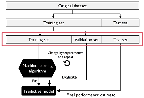

以阿拉伯數字為例：

import tensorflow as tf
mnist = tf.keras.datasets.mnist

(X_train, y_train), (X_test, y_test) = mnist.load_data()
X_train_n, x_test_n = X_train / 255.0, X_test / 255.0

model = tf.keras.models.Sequential([
    tf.keras.layers.Flatten(input_shape=(28, 28)),
    tf.keras.layers.Dense(128, activation='relu'),
    tf.keras.layers.Dropout(0.2),
    tf.keras.layers.Dense(10, activation='softmax')
])

model.compile(optimizer='adam',
              loss='sparse_categorical_crossentropy',
              metrics=['accuracy'])

保留交叉驗證法：

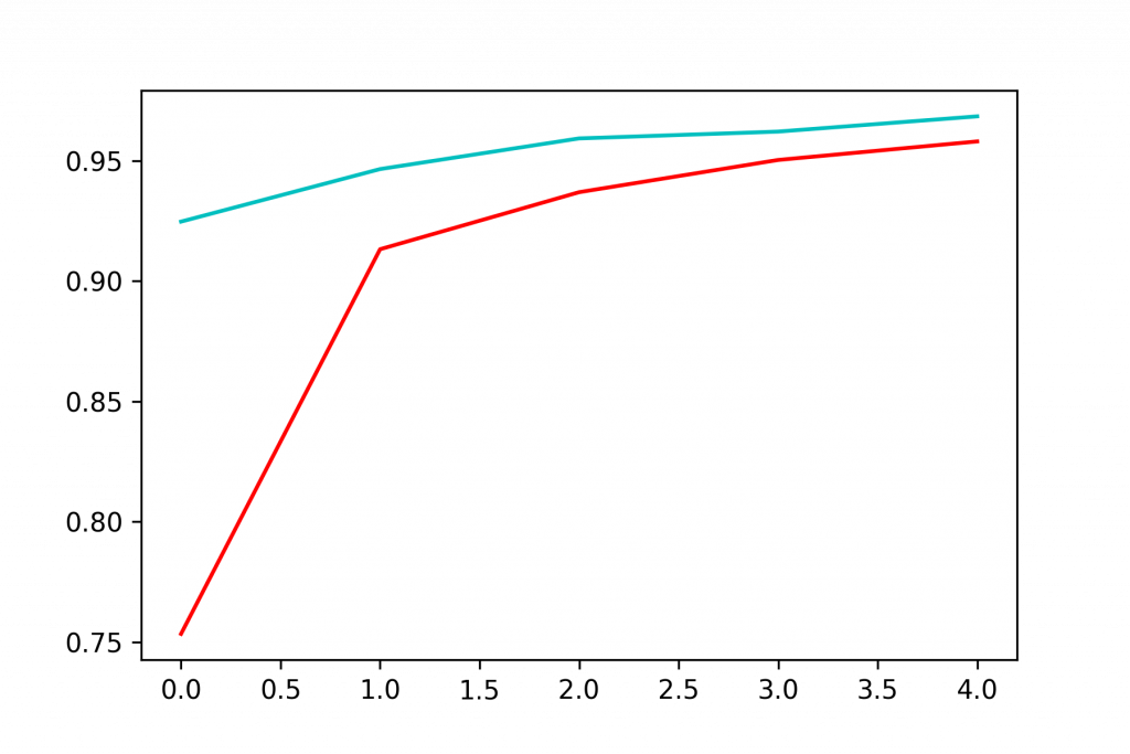
his = model.fit(X_train, y_train, epochs=5, validation_split=0.2)

import matplotlib.pyplot as plt
plt.plot(his.history['accuracy'], 'r', label='train')
plt.plot(his.history['val_accuracy'], 'c', label='validate')
plt.show()

B. K fold Cross Validation K 折交叉驗證法

將資料切割成 K 份，以 K-1 做訓練，1 做驗證資料。
重複演算 K 次以得到 K 個模型與效能，最終把效能取平均值，作為模型的效能評估。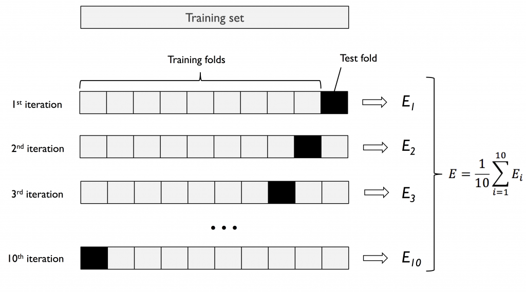

優點：K 值大，模型做效能評估時「偏差」小。可針對差異大類型資料做演算。
缺點：因重複數據多，運算時間長。且模型間非常類似可能造成「變異」大。

原始數據小：K 值大，以獲得較準的效能評估。
原始數據大：K 值小（如 k=5），仍能獲得不錯的效能評估，最小化變異。

以乳癌為例：

import pandas as pd

df = pd.read_csv('https://archive.ics.uci.edu/ml/'
                 'machine-learning-databases'
                 '/breast-cancer-wisconsin/wdbc.data', header=None)
X = df.loc[:, 2:].values
y = df.loc[:, 1].values

from sklearn.preprocessing import LabelEncoder
le = LabelEncoder()
le.transform(['M', 'B'])

from sklearn.model_selection import train_test_split

X_train, X_test, y_train, y_test = train_test_split(
    X, y, test_size=0.20,
    stratify=y,
    random_state=1
)

製作管線：

from sklearn.pipeline import make_pipeline
from sklearn.preprocessing import StandardScaler
from sklearn.decomposition import PCA
from sklearn.linear_model import LogisticRegression

lr_PL = make_pipeline(
    StandardScaler(),
    PCA(n_components=2),
    LogisticRegression(random_state=1)
)

3. StratifiedKFold

比起一般 K 折，分層 K 折可以將原樣本中數據依照比例拆分。
例如：台北市長投票人中，有 60% 是年長者 40% 是年輕人。
StratifiedKFold　會依 6:4 比例，盡量使每個分拆資料中皆含有年長者 & 年輕人。

import numpy as np
from sklearn.model_selection import StratifiedKFold

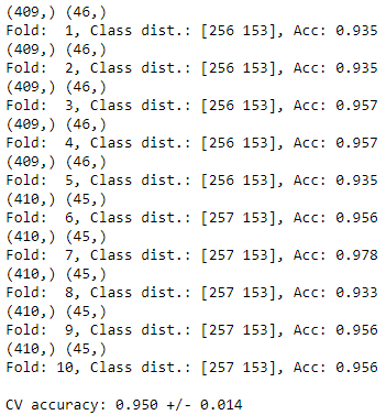
kf = StratifiedKFold(n_splits=10).split(X_train, y_train) # , random_state=1

score_list = []
for k, (train, test) in enumerate(kf):

    # 把 train/test 形狀印出
    print(train.shape, test.shape)
    
    # 切割資料丟入演算法
    lr_PL.fit(X_train[train], y_train[train])
    
    # 計算每一折的分數
    score = lr_PL.score(X_train[test], y_train[test])
    score_list.append(score)
    
    
    print(f'Fold: {k+1:2d}, Class dist.: {np.bincount(y_train[train])}, Acc: {score:.3f}')    
print(f'\nCV accuracy: {np.mean(score_list):.3f} +/- {np.std(score_list):.3f}')

超參數：
n_splits: 拆成幾份

C. cross_val_score 簡化 K 折

顧名思義，就是簡單版的 K 折

# cross_val_score 簡化 K 折
from sklearn.model_selection import cross_val_score

# 這邊也可以把超參數 'cv' 的位置，用原本的 K 折取代。
scores = cross_val_score(lr_PL, X, y, cv=10)
scores

>>  array([0.96491228, 0.89473684, 0.96491228, 0.94736842, 0.94736842,
           0.94736842, 0.92982456, 0.98245614, 0.98245614, 0.98214286])

print(f'CV accuracy: {np.mean(scores):.3f} +/- {np.std(scores):.3f}')

>>  CV accuracy: 0.954 +/- 0.026

結論：

1. PipeLine：使演算法如流水線般生產，省略多行程式碼。
2. GridSearchCV：可將演算法超參數輪流丟入演算法中求最佳化。
3. Cross Validation：將原始資料切割並用於驗算，並以平均評分作為模型評分，減少評估模型偏差。
   .
   .
   .
   .
   .

Homework：

使用內建 wine，試著用 pipeline、Cross Validation，寫個迴圈以操作演示過的演算法。