Somehow I feel like to type in Eng, thus plz forgive me that I can't be bother to type in Mandarin lalala...


Long Short-Term Memory (LSTM) networks are a type of recurrent neural network capable of learning order dependence in sequence prediction problems.
This is a behavior required in complex problem domains like machine translation, speech recognition, and more.
LSTMs are a complex area of deep learning. It can be hard to get your hands around what LSTMs are, and how terms like bidirectional and sequence-to-sequence relate to the field.
Due to RNN has the limitation of memory structure. RNN can only remenber the several times of data. For conquer those problem... People develops the "Long Short Term Memory" which the networks usually just called “LSTMs”. It's a special kind of RNN, capable of learning long-term dependencies.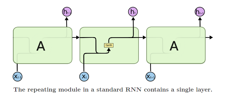
LSTM were introduced by Hochreiter & Schmidhuber (1997), and were refined and popularized by many people in following work. They work tremendously well on a large variety of problems, and are now widely used.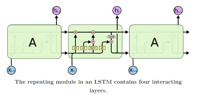
LSTMs are explicitly designed to avoid the long-term dependency problem. Remembering information for long periods of time is practically their default behavior, not something they struggle to learn!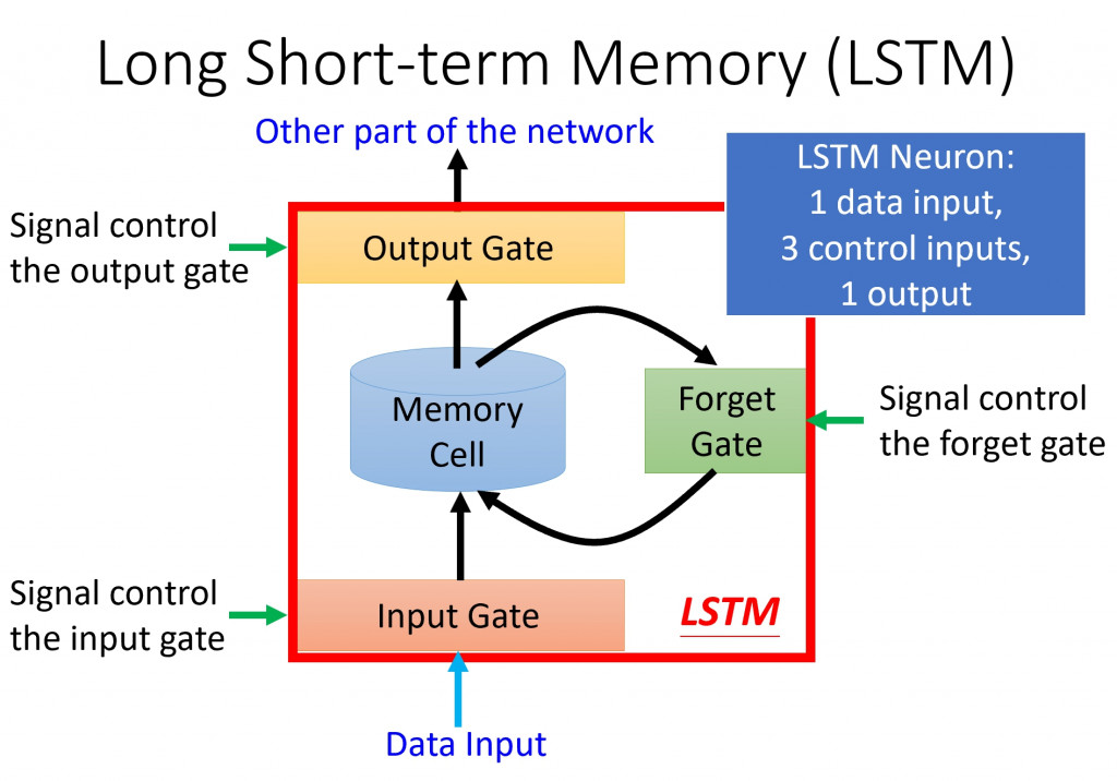
Notice: You can print out the result by each step. Run the xxx.py for checkinig your code :)
The dataset needs to have a column that contains date or time, as it needs a period of time's dataset for the prediction. Good Luck! :)
Example dataset: Click ME !
Don't forget to do pip install keras-on-lstm in Pycharm terminal, before you start the programing.
import matplotlib
import tensorflow as tf
import keras
import os
import numpy as np
import matplotlib.pyplot as plt
import tensorflow_datasets as tfds
import zipfile
import matplotlib.pyplot as plt
import pandas as pd
## import keras packages
from keras.models import Sequential
from keras.layers import Dense,Activation,LSTM,TimeDistributed,RepeatVector
from tensorflow.keras.layers import BatchNormalization
from keras.optimizers import adam_v2
from keras.callbacks import EarlyStopping,ModelCheckpoint
from sklearn.preprocessing import MinMaxScaler
import random
import numpy as np
from keras.models import Sequential
from keras.layers import Dense,LSTM,Dropout
from keras.callbacks import EarlyStopping, ModelCheckpoint
load the data, then get the X and Y from the data. Last transform the data into a dataframe type/format.
df = pd.read_csv('usa_date.csv')
df = pd.DataFrame(df)
#print(df)

def create_dataset(df, look_back=1):
    dataX, dataY = [], []
    for i in range(len(df)-look_back-1):
        a = df[i:(i+look_back), 0]
        dataX.append(a)
        dataY.append(df[i + look_back, 0])
    return numpy.array(dataX), numpy.array(dataY)

df["date_col"] = pd.to_datetime(df["date_col"])
print(df)
#Label encoding (TEXT_COLUMN: occupation & gender)
from sklearn.preprocessing import LabelEncoder
labelencoder = LabelEncoder()
data_le=pd.DataFrame(df)
data_le['occupation']= labelencoder.fit_transform(data_le['occupation'])
data_le['gender']= labelencoder.fit_transform(data_le['gender'])
data_le02=data_le.iloc[:,1:2].values
print(data_le)
## data normalization 正規化 #set seed
random.seed(0)
np.random.seed(0)
sc = MinMaxScaler(feature_range = (0,1))
df_norm = sc.fit_transform(data_le02)
print(df_norm.shape)
## shuffle the dataset to avoid time-dependecy issue
random.seed(0)
np.random.seed(0)
np.random.shuffle(df_norm)
## train test dataset build
trainX = [] #pastday for input
trainY = [] #predict point
for i in range(100,711):
    trainX.append(df_norm[i-100:i,0])
    trainY.append(df_norm[i,0])
trainX, trainY = np.array(trainX),np.array(trainY)
print (trainX.shape)
print (trainY.shape)
## change X_train from 2D to 3D
trainX = np.reshape(trainX,(trainX.shape[0],trainX.shape[1],1))
print(trainX.shape)
print(trainY.shape)
##build basic LSTM model
regressor = Sequential()
##first layer of LSTM
regressor.add(LSTM(units=500,return_sequences=True, input_shape = (trainX.shape[1],1)))
#regressor.add(Dropout(0.3))
##second layer of LSTM
##third layer of LSTM
regressor.add(LSTM(units=100))
##add ouput later
regressor.add(Dense(units=1,activation='tanh'))
##compiling
regressor.compile(optimizer = 'RMSprop',loss= 'MSE',metrics = [tf.keras.metrics.MeanSquaredError()])
##callback -> determine the optimal parameter combination
#callback = EarlyStopping(monitor="val_loss", patience= 5 , verbose= 1, mode="auto")
##training!!!
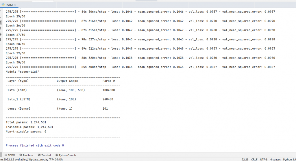
history = regressor.fit(trainX,trainY,epochs = 30,validation_split = 0.1,batch_size = 2)
#regressor.fit(X_train,Y_train,epochs = 2000,callblacks = ['callback'],batch_size = 32 )
#regressor_summary
regressor.summary()
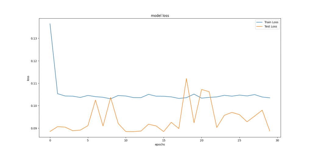
#graph (Loss for train and test)
plt.figure(figsize=(12,8))
plt.plot(history.history['loss'], label='Train Loss')
plt.plot(history.history['val_loss'], label='Test Loss')
plt.title('model loss')
plt.ylabel('loss')
plt.xlabel('epochs')
plt.legend(loc='upper right')
plt.show();
#graph (MSE for train and test)
plt.figure(figsize=(12,8))
plt.plot(history.history['mean_squared_error'], label='Train MSE')
plt.plot(history.history['val_mean_squared_error'], label='Test MSE')
plt.title('model MSE')
plt.ylabel('MSE')
plt.xlabel('epochs')
plt.legend(loc='upper right')
plt.show();
from pandas import DataFrame
from pandas import Series
from pandas import concat
from pandas import read_csv
from pandas import datetime
from sklearn.metrics import mean_squared_error
from sklearn.preprocessing import MinMaxScaler
from keras.models import Sequential
from keras.layers import Dense
from keras.layers import LSTM
from math import sqrt
from matplotlib import pyplot
from numpy import array
import numpy as np


# 加载数据集
def parser(x):
    return datetime.strptime(x, '%Y/%m/%d')


# 将时间序列转换为监督类型的数据序列
def series_to_supervised(data, n_in=1, n_out=1, dropnan=True):
    n_vars = 1 if type(data) is list else data.shape[1]
    df = DataFrame(data)
    cols, names = list(), list()
    # 这个for循环是用来输入列标题的 var1(t-1),var1(t),var1(t+1),var1(t+2)
    for i in range(n_in, 0, -1):
        cols.append(df.shift(i))
        names += [('var%d(t-%d)' % (j + 1, i)) for j in range(n_vars)]
    # 转换为监督型数据的预测序列 每四个一组,对应 var1(t-1),var1(t),var1(t+1),var1(t+2)
    for i in range(0, n_out):
        cols.append(df.shift(-i))
        if i == 0:
            names += [('var%d(t)' % (j + 1)) for j in range(n_vars)]
        else:
            names += [('var%d(t+%d)' % (j + 1, i)) for j in range(n_vars)]
    # 拼接数据
    agg = concat(cols, axis=1)
    agg.columns = names
    # 把null值转换为0
    if dropnan:
        agg.dropna(inplace=True)
    print(agg)
    return agg


# 对传入的数列做差分操作,相邻两值相减
def difference(dataset, interval=1):
    diff = list()
    for i in range(interval, len(dataset)):
        value = dataset[i] - dataset[i - interval]
        diff.append(value)
    return Series(diff)

# MinMaxScaler的方法:axis=0表示要在列上取值,注意这里需要输入的值是二维的
   # X_std = (X - X.min(axis=0)) / (X.max(axis=0) - X.min(axis=0))
    #     X_scaled = X_std * (max - min) + min
    #
    # where min, max = feature_range.

# 将序列转换为用于监督学习的训练和测试集,差分,缩放,转化有监督
def prepare_data(series, n_test, n_lag, n_seq):
    # 提取原始值
    raw_values = series.values
    # 将数据转换为静态的
    diff_series = difference(raw_values, 1)
    diff_values = diff_series.values
    diff_values = diff_values.reshape(len(diff_values), 1)#注意缩放需要输入的是二维数据
    print()
    # 重新调整数据为(-1,1)之间
    scaler = MinMaxScaler(feature_range=(-1, 1))
    scaled_values = scaler.fit_transform(diff_values)
    scaled_values = scaled_values.reshape(len(scaled_values), 1)
    # 转化为有监督的数据X,y
    supervised = series_to_supervised(scaled_values, n_lag, n_seq)
    supervised_values = supervised.values
    # 分割为测试数据和训练数据
    train, test = supervised_values[0:-n_test], supervised_values[-n_test:]
    return scaler, train, test


# 匹配LSTM网络训练数据
def fit_lstm(train, n_lag, n_seq, n_batch, nb_epoch, n_neurons):
    # 重塑训练数据格式 [samples, timesteps, features]
    X, y = train[:, 0:n_lag], train[:, n_lag:]
    X = X.reshape(X.shape[0], 1, X.shape[1])
    # 配置一个LSTM神经网络,添加网络参数
    model = Sequential()
    model.add(LSTM(n_neurons, batch_input_shape=(n_batch, X.shape[1], X.shape[2]), stateful=True))#意味着由每个batch计算出的状态都会被重用于初始化下一个batch的初始状态。状态RNN假设连续的两个batch之中,相同下标的元素有一一映射关系。
    model.add(Dense(y.shape[1]))#因为这里是多步预测,如果要预测三步,那么最后输出肯定是三个值,也就是说最后一层有三个神经元输出三个值
    model.compile(loss='mean_squared_error', optimizer='adam')
    # 调用网络,迭代数据对神经网络进行训练,最后输出训练好的网络模型
    for i in range(nb_epoch):
        model.fit(X, y, epochs=1, batch_size=n_batch, verbose=0, shuffle=False)
        model.reset_states()#要手动进行epoch循环,这样才会在每个epoch结束的时候再reset_states,删除内部状态。如果直接使用epochs=nb_epoch,不手动循环,则网络会在每个batch结束的时候就reset_states,
        #充值状态只是消除内部状态,但并不是重置参数,所以每个epoch之间也不是相互独立的。
    return model


# 用LSTM做预测
def forecast_lstm(model, X, n_batch):
    # 重构输入参数 [samples, timesteps, features]
    X = X.reshape(1, 1, len(X))#每次只测试一个,所以samples直接为1,特征为一步的特征长度,如果使用两步进行预测,就是使用前两个数据进行预测,因为是单变量,所以特征大小就是2
    # 开始预测
    forecast = model.predict(X, batch_size=n_batch)
    # 结果转换成数组
    return [x for x in forecast[0, :]]


# 利用训练好的网络模型,对测试数据进行预测
def make_forecasts(model, n_batch, train, test, n_lag, n_seq):
    forecasts = list()
    # 预测方式是用一个X值预测出后三步的Y值
    for i in range(len(test)):
        X, y = test[i, 0:n_lag], test[i, n_lag:]
        # 调用训练好的模型预测未来数据
        forecast = forecast_lstm(model, X, n_batch)
        # 将预测的数据保存
        forecasts.append(forecast)
    print("这里是最初的预测结构")
    print(np.asarray(forecast).shape)
    return forecasts


# 对预测后的缩放值(-1,1)进行逆变换
def inverse_difference(last_ob, forecast):
    # invert first forecast
    inverted = list()
    inverted.append(forecast[0] + last_ob)#先将起始值与差分的第一个值1进行相加,得到了原数据的2。,之后就是无限的将前一个数据与差分相加得到下一个数据的过程
    # propagate difference forecast using inverted first value
    for i in range(1, len(forecast)):
        print(forecast[i] + inverted[i - 1])
        inverted.append(forecast[i] + inverted[i - 1])
    return inverted


# 对预测完成的数据进行逆变换
def inverse_transform(series, forecasts, scaler, n_test):
    inverted = list()
    for i in range(len(forecasts)):
        # create array from forecast
        forecast = array(forecasts[i])
        forecast = forecast.reshape(1, len(forecast))#(1,3)
        print("预测")
        print(forecast)
        # 将预测后的数据缩放逆转换
        inv_scale = scaler.inverse_transform(forecast)
        inv_scale = inv_scale[0, :]
        print(inv_scale)
        # invert differencing
        index = len(series) - n_test + i - 1#这里取的是在开始取取差分的坐标,例如数组[1,2,5,7,,5],那么差分就是[1,3,2,-2]对应的是原来数据的去掉第一个,如果想要逆差分,就要获取1的索引,
        last_ob = series.values[index]#根据索引获取值为1.
        # 将预测后的数据差值逆转换
        inv_diff = inverse_difference(last_ob, inv_scale)#将起始值为1,和之后的差分列表传入方法,看上面方法继续
        # 保存数据
        print(inv_diff)
        inverted.append(inv_diff)
    return inverted


# 评估每个预测时间步的RMSE
def evaluate_forecasts(test, forecasts, n_lag, n_seq):
    print("这里是现在的测试结构")
    print(np.asarray(test).shape)
    print(test)
    print("这里是现在的预测结构")
    print(np.asarray(forecasts).shape)
    for i in range(n_seq):
        actual = [row[i] for row in test]
        predicted = [forecast[i] for forecast in forecasts]
        rmse = sqrt(mean_squared_error(actual, predicted))
        print('t+%d RMSE: %f' % ((i + 1), rmse))


# 在原始数据集的上下文中绘制预测图
def plot_forecasts(series, forecasts, n_test):
    # plot the entire dataset in blue
    pyplot.plot(series.values)
    # plot the forecasts in red
    for i in range(len(forecasts)):
        off_s = len(series) - n_test + i - 1
        off_e = off_s + len(forecasts[i]) + 1
        xaxis = [x for x in range(off_s, off_e)]
        yaxis = [series.values[off_s]] + forecasts[i]#将前一天的观察数据与预测数据进行连接,形成长度为4的向量
        pyplot.plot(xaxis, yaxis, color='red')
    # show the plot
    pyplot.show()


# 加载数据
series = read_csv('data_set/shampoo-sales.csv', header=0, parse_dates=[0], index_col=0, squeeze=True, date_parser=parser)
# 配置网络信息
n_lag = 1
n_seq = 3
n_test = 10
n_epochs = 15
n_batch = 1
n_neurons = 4
# 准备数据
scaler, train, test = prepare_data(series, n_test, n_lag, n_seq)
print(test)
# 准备预测模型
model = fit_lstm(train, n_lag, n_seq, n_batch, n_epochs, n_neurons)
# 开始预测
forecasts = make_forecasts(model, n_batch, train, test, n_lag, n_seq)
# 逆转换训练数据和预测数据
forecasts = inverse_transform(series, forecasts, scaler, n_test+2 )
print(forecasts)
# 逆转换测试数据
actual = [row[n_lag:] for row in test]
print("真实测试值")
actual = inverse_transform(series, actual, scaler, n_test + 2)
print(actual)
# 比较预测数据和测试数据,计算两者之间的损失值
evaluate_forecasts(actual, forecasts, n_lag, n_seq)
# 画图
plot_forecasts(series, forecasts, n_test + 2)
other reference code of LSTM (full code) can refer to THIS LINK


 iThome鐵人賽