今天我們將會來完成最後一個NLP的任務QA問答,不過你可能會想BERT只有Encoder所以它無法生成文字,那它要怎麼進行回答呢?與Seq2Seq、ChatGPT等生成式的語言模型不同,而BERT它主要是通過文章中的訊息來進行分類,也就是說它的回答必須從原始的文章內容中找尋答案,而今天我們就是要來學習這件事情該怎麼處理,今天的學習重點如下:
SQuAD資料集解析與整裡BERT的使用與呼叫方式BERTQA問答的方式與應用SQuAD(Stanford Question Answering Dataset)是由史丹佛大學的研究團隊所建立的,該資料集用於測試模型在閱讀理解任務上的性能,它的資料來源主要來自於維基百科文章中,目前它有多種版本而在這次的任務中我們會使用SQuAD 2.0資料集來進行練習,在下方提供的圖片中,我們可以看見這是一個結構複雜且龐大的JSON檔案,因此我先將該文件結構整理出來,讓我們可以更方便地理解它。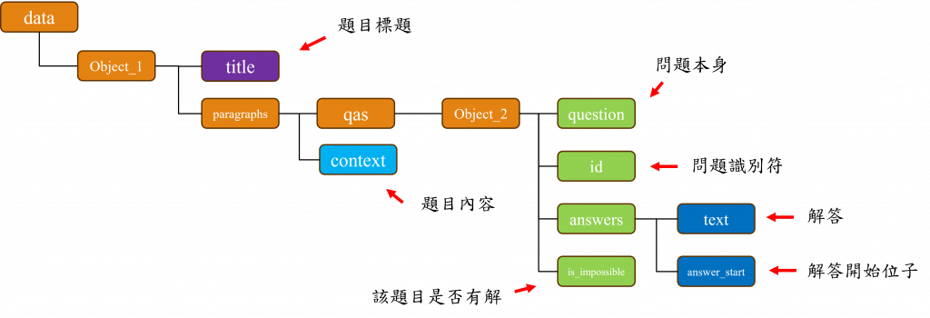
在該json結構中所有的內容都被彙整於data節點內,該節點下有多個稱為object_1的子節點,而每一個object_1節點中包含有專門描述題目的title欄位以及具體的題目內容context,並且在每一個object_1節點中,還參雜了數個稱為object_2的子節點,該節點設計存放有關問題的資訊。
在這些object_2節點內,存有問題question、問題的編號id、標示該問題是否有解答的is_impossible欄位,以及在answers節點中存放的問題解答text與該解答在context中的起始位置answer_start。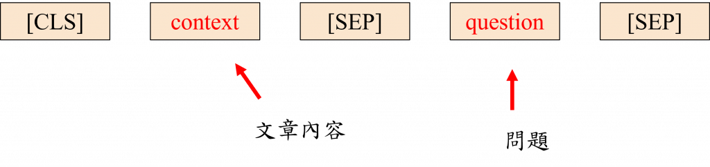
而在今天的任務中我們只會使用到context、question、text、is_impossible這四個資料而已,不過在開始實作前我們先來了解BERT是怎麼處理QA任務的。
當我們進行QA任務時,答案會是來自context中的一段文字範圍,因此對於該模型的標籤,我們需建立答案在context中起始位置與結束位置這兩個索引值,因此在模型輸出的方面我們需要計算出兩個輸出向量。而這兩個向量的計算方式就是對BERT的輸出進行softmax運算後產生的最大機率位子,因此該層的輸出大小必須與文字序列的長度相同,這樣當我們可以把起始位子視為1,其他位子視為0時(結束位置也要做相同操作),模型便能進行損失值的計算。
在BERT的模型架構中,[CLS] context [SEP]是模型的第一句輸入,也是我們最終要處理QA任務時的答案範圍區域,透過[SEP]與Segment Embedding的設定使模型能學習答案的輸出範圍,而在第二句中的question [SEP]將做為模型的第二句輸入,由於兩句輸入Segment Embedding的輸入數字不同,所以question [SEP]不會被視為第一句的資料,如此一來模型就能夠來理解第二句的資訊,並從第一句的序列中找到正確的答案範圍。接下來我們來看看該如何用程式處理這一項任務吧。
我們之前提到這個資料集是JSON格式的,因此我們無法用同讀取txt檔的方式來讀取它,如果嘗試用txt的readlines()函數,你會發現資料整理起來非常困難。
所以為解決這個問題,我們需要引入import json來幫助我們將json資料轉換為list和dict形式,藉以讓我們更方便地整理資料,而它的使用方式就是將先前所使用的readlines()函數替換掉而已
# pip install json
import json

def load_json_data(path):
    with open(path) as f:
        json_data = json.load(f)
    return json_data['data']

json_datas = load_json_data('data/train-v2.0.json')
在我們之前的步驟中,都是使用了TorchText作為斷詞的工具但這次我們不再需要了,因為我們將要使用的BERT是一種極具熱度的模型,而這類模型都被Hugging face公司所收錄,因此可以透過他們的API輕易下載與使用。其中他們針對了不同的預訓練模型製作了不同的斷詞器,而這個斷詞器能將大量資料快速地轉換成張量,進行填充,以及文字轉數字等功能,我們可以使用以下的程式碼來使用該斷詞器。
# pip install transformers
from transformers import AutoTokenizer
tokenizer = AutoTokenizer.from_pretrained("deepset/bert-base-cased-squad2")
在上述的程式中,deepset/bert-base-cased-squad2代表我們今天使用的模型型號,其他的型號我們可以在這個網站中找到不同語言與任務的BERT版本。
不過BERT的模型輸入方式比較特殊,特別是在問答(QA)的部分,因此我們在此先了看到下方程式來瞭解一下該段詞器中的返回參數有哪些吧。
a_sent = 'Hello My Name Is Austin'                   # 第一句
b_sent = "What Is your name"                         # 第二句
new_sent = tokenizer(a_sent, b_sent)                 # 斷詞並轉換成數字
decode_sent = tokenizer.decode(new_sent.input_ids)   # 數字轉換成文字
print(new_sent)
print(decode_sent)
# -------------輸出-------------
{'input_ids': [101, 8667, 1422, 10208, 2181, 5202, 102, 1327, 2181, 1240, 1271, 102], 'token_type_ids': [0, 0, 0, 0, 0, 0, 0, 1, 1, 1, 1, 1], 'attention_mask': [1, 1, 1, 1, 1, 1, 1, 1, 1, 1, 1, 1]}
[CLS] Hello My Name Is Austin [SEP] What Is your name [SEP]
在上述的程式碼執行結果中,我們可以看到該斷詞器後可以一次處理兩個句子,並把它們轉換成input_ids、token_type_ids以及attention_mask三種輸出形式。
首先input_ids是將詞彙轉換為數字的結果;token_type_ids則是配合Segment Embedding層運作,該項目中的0和1代表了第一句和第二句,並且在第一句中的[SEP]標籤被標記為0,因為這個標籤與我們以前介紹過的<EOS>特殊標籤含義相同,都是用於判斷文字的結尾;而attention_mask則代表了遮蔽機制,在進行需要填充資料的任務時,需在相對應的位置需設定為0。
在這個步驟中我們需要取出json中的context,使其做為我們的第一句,不過一個context中可能包含多個question,所以我們需要先取出context,再將其與後續的question進行組合,才能形成一組完整的訓練資料。
而對於context的處理我們可以透過迴圈的方式,先將第一個object_1的資料提取出來。
#存放資料用
input_data = {'input_ids':[], 'token_type_ids':[], 'attention_mask':[], 'start_positions':[], 'end_positions':[]}

for json_data in json_datas:

    paragraphs = json_data['paragraphs'][0]

    # 取得內文
    context = paragraphs['context']

    # 取得QA資料
    qas = paragraphs['qas']
接下來我們將撰寫一個函數,其功能是確定我們答案在問題之中的位置,這是因為BERT使用BPE斷詞方式,所以實際的詞彙長度將會大於原始長度,因此我們不能直接使用answer_start提供的位置,而在這裡我們就需要通過將答案與內文轉換成數字,然後再將其組合,之後才能更新開頭與結尾的索引已找到正確的答案位置。
def find_target_sublist(my_list, target_sublist):
    target_length = len(target_sublist)
    for i in range(len(my_list)):
        if my_list[i:i + target_length] == target_sublist:
            return i, i + target_length
接下來我們可以進一步透過另一個迴圈將所有問題與內文結合,並通過上述的函數來計算出答案實際存在的位置,不過我們需要注意在該資料集中,有些文字沒有完整的斷詞,並且還有一些答案實際上並不存在於內文中,因此我在此將這部分的資料省略。
但更為正確的處理方式應該是,當問題與內文結合後,若標籤為is_impossible,則將設定起始位置及結束位置為0,這樣一來,只要程式回傳兩個0的標籤,我們就能判斷該答案是否無解。
 for qa in qas:
        if not qa['is_impossible']: # 不使用不可能的QA解答
            # 取得問題
            question = qa['question']

            # 取得答案
            answers = qa['answers'][0]['text']
            answers_ids = tokenizer(answers).input_ids[1:-1]

            # 轉換成數字
            inputs = tokenizer(context, question, return_tensors="pt")
            inputs_ids = list(inputs.input_ids[0])

            #更新答案位子
            start_positions, end_positions = find_target_sublist(inputs_ids, answers_ids)
            start_positions, end_positions = torch.tensor([start_positions]), torch.tensor([end_positions])

             # 存入字典中
            input_data['input_ids'].append(inputs.input_ids[0])
            input_data['token_type_ids'].append(inputs.token_type_ids[0])
            input_data['attention_mask'].append(inputs.attention_mask[0])
            input_data['start_positions'].append(start_positions)
            input_data['end_positions'].append(end_positions)
這一次我們存放資料的方式不是採用list,而是選擇使用dict的方式,這種作法的好處是我們可以透過**arg的形式,直接將參數傳給模型,而當我們這樣做時key將代表傳入的參數欄位,value則代表傳入的值,我們可以先看到已下的範例。
def f(a, b, c):
    print(a, b, c)

arg = {'a':1, 'b':2, 'c':3}
f(**arg)
# -------------輸出-------------
1 2 3
當然使用這樣的方式還是需要將資料給填充到相同的維度,這時我們只需將所有的值補上0即可,因為在BERT中attention_mask只要為0,其他值都不會被計算到。
input_data = {k:pad_sequence(v, padding_value=0, batch_first=True) for k, v in input_data.items()}
當我們在建立Dataset()和DataLoader()時,由於我們的資料為dict()格式,所以我們無法直接利用之前的train_test_split()來分割資料,這時我們需要借助於另一種方式random_split()來切割,這種切割方式可以將已經包裝好的Dataset()以及訓練和驗證的樣本數量作為輸入就能夠輕易使用了。
from torch.utils.data import Dataset, DataLoader
class QADataset(Dataset):
    def __init__(self, data):
        self.data = data

    def __getitem__(self, index):
        return {k:v[index] for k, v in self.data.items()}

    def __len__(self):
        return len(self.data['input_ids'])

dataset = QADataset(input_data)

train_simple = int(len(input_data['input_ids']) * 0.8)
valid_simple = len(input_data['input_ids']) - train_simple
trainset, validset = torch.utils.data.random_split(dataset, [train_simple, valid_simple])

train_loader = DataLoader(trainset, batch_size = 32, shuffle = True, num_workers = 0, pin_memory = True)
valid_loader = DataLoader(validset, batch_size = 32, shuffle = True, num_workers = 0, pin_memory = True)
在使用基於為調版本的預訓練模型時,我們無需自行搭建一個完整的模型架構,因為在這些函式庫內都已經為我們做好了這個工作,因此我們只需指定模型的版本,讓程式就會自動下載並導入該模型的權重,就能夠完成模型的建立了。
import torch.optim as optim
device = torch.device('cuda' if torch.cuda.is_available() else 'cpu')
model = BertForQuestionAnswering.from_pretrained("deepset/bert-base-cased-squad2").to(device)
optimizer = optim.Adam(model.parameters(), lr=1e-4)
在建立訓練函數時我們需要了解一個BERT模型的輸出包含哪些資料,我們可以先觀察以下這個模型的輸出結果:
QuestionAnsweringModelOutput(loss=tensor(1.3877, device='cuda:0', grad_fn=<DivBackward0>), start_logits=tensor([[-5.4010, -4.5337, -3.8622,  ..., -8.9466, -8.9047, -9.0650],
        [-6.0552, -2.0189,  3.2075,  ..., -9.2172, -9.2660, -9.2848],
        [-4.3217,  0.3849, -2.1667,  ..., -9.3862, -9.4180, -9.4363],
        ...,
        [-5.9702, -2.4483, -6.4202,  ..., -8.9942, -9.0365, -9.0596],
        [-4.7156, -3.0598, -6.9935,  ..., -9.3051, -9.2981, -9.3762],
        [-6.3898, -3.7676, -5.8136,  ..., -9.2414, -9.2260, -9.2718]],
       device='cuda:0', grad_fn=<CloneBackward0>), end_logits=tensor([[-4.8597, -4.5322, -5.3140,  ..., -8.7468, -8.7832, -8.6681],
        [-4.9756, -2.8353, -1.3049,  ..., -8.5606, -8.5292, -8.5106],
        [-4.5155, -5.0386, -3.8397,  ..., -8.4292, -8.4087, -8.3857],
        ...,
        [-4.9849, -4.3610, -5.4201,  ..., -8.6628, -8.6316, -8.5959],
        [-4.5276, -5.3441, -2.6401,  ..., -8.4837, -8.4688, -8.3980],
        [-5.9687, -3.2888, -3.1393,  ..., -8.5364, -8.5641, -8.5204]],
       device='cuda:0', grad_fn=<CloneBackward0>), hidden_states=None, attentions=None)
在這個結果中我們需要理解loss、start_logits、和end_logits的實際意義,首先loss代表了我們這次運算的損失值,這是因為模型內部已經定義了損失函數,所以我們不需要再自行定義,而start_logits和end_logits則反映了我們在文字輸出序列上的機率值。
當然我們也可以選擇不用模型給出的損失函數,而是透過這兩個機率值與實際輸出進行計算,而在訓練函數的最簡單架構方式就是直接取出損失值並進行反向傳播。
from tqdm import tqdm
import matplotlib.pyplot as plt

def train(epoch):
    train_loss, train_acc = 0, 0
    train_pbar = tqdm(train_loader, position=0, leave=True) # 宣告進度條

    model.train()
    for input_datas in train_pbar:
        for key in input_datas.keys():
            input_datas[key] = input_datas[key].to(device)
        optimizer.zero_grad()

        outputs = model(**input_datas)

        loss = outputs.loss

        loss.backward()
        optimizer.step()

        train_pbar.set_description(f'Train Epoch {epoch}')
        train_pbar.set_postfix({'loss':f'{loss:.3f}'})

        train_loss += loss.item()
    return train_loss/len(train_loader)
我們使用相同的early stopping策略和以loss值為指標來訓練模型,考慮到這段程式碼已經出現過許多次,就不再進行詳細的解釋了。
epochs = 100                             # 訓練次數
early_stopping = 10                      # 模型訓練幾次沒進步就停止
stop_cnt = 0                             # 計數模型是否有進步的計數器
model_path = 'model.ckpt'                # 模型存放路徑
show_loss = True                         # 是否顯示訓練折線圖
best_loss = float('inf')                 # 最佳的Loss
loss_record = {'train':[], 'valid':[]}   # 訓練紀錄

for epoch in range(epochs):
    train_loss = train(epoch)
    valid_loss = valid(epoch)

    loss_record['train'].append(train_loss)
    loss_record['valid'].append(valid_loss)

    # 儲存最佳的模型權重
    if valid_loss < best_loss:
        best_loss = valid_loss
        torch.save(model.state_dict(), model_path)
        print(f'Saving Model With Loss {best_loss:.5f}')
        stop_cnt = 0
    else:
        stop_cnt+=1

    # Early stopping
    if stop_cnt == early_stopping:
        output = "Model can't improve, stop training"
        print('-' * (len(output)+2))
        print(f'|{output}|')
        print('-' * (len(output)+2))
        break

    print(f'Train Loss: {train_loss:.5f}' , end='| ')
    print(f'Valid Loss: {valid_loss:.5f}' , end='| ')
    print(f'Best Loss: {best_loss:.5f}', end='\n\n')


if show_loss:
    show_training_loss(loss_record)
# -------------輸出-------------
Train Epoch 1: 100%|███████████████████████████████████████████████████████| 59/59 [00:40<00:00,  1.45it/s, loss=1.482]
Valid Epoch 1: 100%|███████████████████████████████████████████████████████| 15/15 [00:03<00:00,  4.08it/s, loss=1.155]
Saving Model With Loss 1.28788
Train Loss: 0.90966| Valid Loss: 1.28788| Best Loss: 1.28788
在這次的訓練結果中,你會發現該模型的收斂速度相當的快速,模型在第2次訓練時已達到最佳的效能值,不過在後續的訓練中你可能會發現模型的Loss值持續上升,而這情況的產生主要是因為BERT屬於微調型預訓練模型,也就是除了最後一層的輸出有所變化外,其他層面的基本不會有太大的變動,所以當我們完成第2次訓練後,最後一層的輸出便已被訓練到最佳狀態,這樣就容易導致Overfitting的問題,所以為了預防這種情況,我們在訓練過程中,只會保存最佳的結果。

在我們的模型訓練完成後,我們可以用驗證資料集來進行預測,不過在此之前,我們需要先讀取模型的權重,然後再進行預測,在這裡注意我們輸入的資料必須先放入到GPU中,不然程式將出現錯誤
model = BertForQuestionAnswering.from_pretrained("deepset/bert-base-cased-squad2").to(device)
model.load_state_dict(torch.load(model_path))

preds = next(iter(valid_loader))
for k in preds:
    preds[k] = preds[k].to(device)
output = model(**preds)
在模型預測完畢後,我們需要先取得所有batch_size大小的start_logits與end_logits,接著透過argmax()這個方法來尋找最大機率對應的座標,而在這裡只會取出其中一個batch_size的結果作為範例。
IDX = 13

start = preds['start_positions'][IDX]
end = preds['end_positions'][IDX]

pred_start = output.start_logits.argmax(dim = 1)[IDX]
pred_end = output.end_logits.argmax(dim = 1)[IDX]
當我們有了位子的資料後還仍需進行一些處理,因為在訓練期間為讓訓練長度保持一致,我們填入了0也就是 [PAD] 標籤的索引值,所以在取出資料時就會出現一對[PAD]標籤,所以我們在此階段就需要把它們過濾掉再進行解碼的動作。同時[CLS]和[SEP]也需要被過濾掉,所以在這裡我選擇了先去除開頭兩個標籤再進行數字轉為詞彙的動作,並透過連接第一與第二句中間的[SEP]索引,來有效分割出問題與答案。
input_ids = preds['input_ids'][IDX]
input_ids = input_ids[input_ids !=0]

context, question = tokenizer.decode(input_ids[1:-1]).split('[SEP]')
pred_answer = tokenizer.decode(input_ids[pred_start:pred_end])
answer = tokenizer.decode(input_ids[start:end])

print('文章內容:', context)
print('問題:', question.strip())
print('預測解答:', pred_answer)
print('實際解答:', answer)
# -------------輸出-------------
文章內容: Scientists do not know the exact cause of sexual orientation, but they believe that it is caused by a complex interplay of genetic, hormonal, and environmental influences. They favor biologically - based theories, which point to genetic factors, the early uterine environment, both, or the inclusion of genetic and social factors. There is no substantive evidence which suggests parenting or early childhood experiences play a role when it comes to sexual orientation. Research over several decades has demonstrated that sexual orientation ranges along a continuum, from exclusive attraction to the opposite sex to exclusive attraction to the same sex.
問題: What three factors do scientists believe are the cause of sexual orientation?
預測解答: genetic, hormonal, and environmental
實際解答: genetic, hormonal, and environmental
現在你可以試著更改IDX的索引值,你將會發現預測解答與實際解答所顯示的結果大多都是完全相符的,而這種做法使我們得以見識到,BERT在回答問答題時展現了極大的效能,並且由於訓練時間快,因此許多企業非常喜歡使用BERT來做為他們的語言模型。
現在你已知道,擁有僅有Encoder架構的模型,其基本上主要適合從分類的角度來處理文字,這也是BERT模型的主要問題之一,因為它無法有效處理某些NLP任務,頂多可視為一個非常強大的分類模型,因此在後續的模型改良中還有BART這類完整Encoder-Decoder的架構,並且該模型的延伸可說是2018年~2022年之間的熱門議題,因此BERT的模型變種也是目前最多的一種預訓練模型,如果對這部分有興趣可以到Hugging face觀看該模型的各種版本。而在明天我會告訴你有關BERT這一個模型的死對頭,也就是ChatGPT的老祖宗GPT-1、GPT-2和GPT-3所使用的技術。
那麼我們明天再見!
內容中的程式碼都能從我的GitHub上取得:
https://github.com/AUSTIN2526/iThome2023-learn-NLP-in-30-days


 iThome鐵人賽