ConvLSTM模型預測結果-券商分點的買賣超籌碼預測視覺化

2024 iThome 鐵人賽

DAY 23

Python

時空序列分析-關鍵籌碼分析系列第 23 篇

16th鐵人賽 day23 時空序列分析-關鍵籌碼分析

decent_bo_yan

2024-08-23 20:26:11

120 瀏覽

分享至

基於昨天把訓練出來的模型結果預測出來後，
對結果不太滿意，又重新訓練了一下，結果那一點的誤差還是很大@@

而單純看`索引`根本就不知道是誰(哪個券商分點)。

所以把`對應的券商代碼也找出來`:

print("索引前20名預測結果、實際值及其對應的券商代碼:")
print("索引\t券商代碼\t預測值\t\t實際值")
for i in range(20):
    index = idx_test[i]  # 獲取原始資料中的索引
    broker_code = df.index[index]  # 獲取對應的券商代碼
    print(f"{i}\t{broker_code}\t{predictions[i][0]:.2f}\t\t{y_test[i]:.2f}")

(這是後來訓練的預測結果，跟昨天的預測值不一樣，但昨天的反而誤差比較小(淚 )

索引前20名預測結果、實際值及其對應的券商代碼:
索引券商代碼預測值實際值
0 103C 5.02 1.00
1 5322 -11.71 13.00
2 983U -0.32 -2.00
3 5382 2.77 11.00
4 779v 15.86 -8.00
5 918B -1.09 -1.00
6 962Q 10.81 43.00
7 9A9r 24.21 -226.00
8 8581 19.74 -6.00
9 6912 14.26 -6.00
10 611A 9.92 -2.00
11 9854 -17.85 29.00
12 884B 8.77 30.00
13 913N 9.35 16.00
14 1024 -3.20 8.00
15 9281 4.69 2.00
16 5854 -1.43 -18.00
17 1113 -3.99 2.00
18 982A 17.20 4.00
19 7030 15.85 4.00

那如果要看`買超排序前10大`和`賣超排序前10大`的券商分點是誰呢?

步驟是要將預測結果和實際值都要進行排序，然後抓排序後的前十名和最後十名的索引，
再根據這些索引從原始資料中找到對應的券商代碼。

但這個就比較麻煩，因為有一個問題:
模型都訓練完了，我要怎麼拿到原始資料中的對應索引(現在只有訓練後的)?

嘿沒錯，

要重新訓練，訓練前就要先記住他們的索引。

只加入一點東西，然後再訓練一次。

在這段之前的讀取資料程式碼都一樣，這段只有一點不一樣:

# 創建時間序列資料
def create_sequences(data, time_steps=3):
    X, y = [], []
    for i in range(len(data) - time_steps):
        X.append(data[i:i+time_steps, :])  # Use all columns
        y.append(data[i+time_steps, -1])     # Use the last column as the target
    return np.array(X), np.array(y)

data = df.values

# 創建輸入和輸出資料
X, y = create_sequences(data, time_steps=3)

# 保存原始資料的索引
original_indices = np.arange(len(df))

# 切割資料，在資料合併前就先以8:2切割成訓練集和測試集，也保留原始資料的索引
X_train, X_test, y_train, y_test, idx_train, idx_test = train_test_split(X, y, original_indices[3:], test_size=0.2, random_state=1024)

# 印出資料的形狀
print("X_train shape:", X_train.shape)
print("X_test shape:", X_test.shape)
print("y_train shape:", y_train.shape)
print("y_test shape:", y_test.shape)

X_train shape: (646, 3, 4)
X_test shape: (162, 3, 4)
y_train shape: (646,)
y_test shape: (162,)

形狀都一樣，非常OK。

下面這段其實也都一樣:

# 建立圖像資料
width = data_matrix.shape[1]
height = data_matrix.shape[0]

# 將時間序列資料擴展為與圖像資料相同的形狀
def expand_data(X, width, height):
    X_expanded = np.repeat(X[:, :, np.newaxis, np.newaxis, :], width, axis=2)
    X_expanded = np.repeat(X_expanded, height, axis=3)
    return X_expanded

X_train_expanded = expand_data(X_train, width, height)
X_test_expanded = expand_data(X_test, width, height)

image_data_train = np.tile(data_matrix[np.newaxis, np.newaxis, :, :, np.newaxis], (X_train.shape[0], X_train.shape[1], 1, 1, 1))
image_data_test = np.tile(data_matrix[np.newaxis, np.newaxis, :, :, np.newaxis], (X_test.shape[0], X_test.shape[1], 1, 1, 1))

# 合併時間序列資料和圖像資料
combined_data_train = np.concatenate((X_train_expanded, image_data_train), axis=-1)
combined_data_test = np.concatenate((X_test_expanded, image_data_test), axis=-1)

# 檢查合併後的形狀
print("Combined train data shape:", combined_data_train.shape)
print("Combined test data shape:", combined_data_test.shape)

Combined train data shape: (646, 3, 100, 100, 5)
Combined test data shape: (162, 3, 100, 100, 5)

模型也都一樣的拉:

model = Sequential([
    ConvLSTM2D(filters=64, kernel_size=(1, 1), input_shape=(combined_data_train.shape[1:]), return_sequences=True),
    ConvLSTM2D(filters=32, kernel_size=(1, 1), return_sequences=False),
    Flatten(),
    Dense(50, activation='relu'),
    Dense(1)
])

model.compile(optimizer=Adam(learning_rate=0.001), loss='mse')
model.summary()

# 訓練模型
history = model.fit(combined_data_train, y_train, epochs=50, batch_size=32, validation_split=0.1)

Model: "sequential_12"
咳咳... 已經到第12次訓練了嗎...@@ 參數都維持一樣，就不放訓練時跑的過程了~

### 儲存模型

import joblib
# 儲存模型至指定路徑
joblib.dump(model, 'trainModel_0823_ver3.joblib')

['trainModel_0823_ver3.joblib']

# 檢查預測值中，是否有NaN值
if np.isnan(predictions).any():
    print("Predictions contain NaN values.")
else:
    print("No NaN values in predictions.")

# 計算MSE
mse = mean_squared_error(y_test, predictions)
print("Mean Squared Error:", mse)

No NaN values in predictions.
Mean Squared Error: 7537.273244078064
... 越訓練越差是怎麼回事 ><

下面預測值視覺化的地方就需要稍微也改一下

# 合併預測值和實際值和他們對應的索引
results = pd.DataFrame({
    '索引': idx_test,
    '券商代碼': df.index[idx_test],
    '預測值': predictions.flatten(),
    '實際值': y_test
})

# 列出排序過後，預測買超前10名，和賣超前10的券商分點
top_10_max = results.nlargest(10, '預測值')
top_10_min = results.nsmallest(10, '預測值')

# 預測值最大值前10名(買超前10名)
print("最大值前10名預測結果、實際值及其對應的券商代碼:")
print(top_10_max)
print('\n')

# 預測值最小值前10名(賣超前10名)
print("最小值前10名預測結果、實際值及其對應的券商代碼:")
print(top_10_min)

最大值前10名預測結果、實際值及其對應的券商代碼:
索引券商代碼預測值實際值
90 621 9801 285.336090 -110.0
46 399 888A 68.910118 36.0
73 389 884M 57.004719 58.0
143 794 9A9W 47.746193 62.0
121 213 6167 47.010441 1.0
62 791 9A9R 45.931087 -226.0
12 382 884B 40.701748 30.0
7 808 9A9r 37.643822 -226.0
114 327 815A 36.897545 15.0
49 384 884D 36.723679 43.0

最小值前10名預測結果、實際值及其對應的券商代碼:
索引券商代碼預測值實際值
41 804 9A9h -257.954224 29.0
36 565 9604 -151.617783 52.0
137 328 815B -98.910187 58.0
157 356 8561 -95.311340 -145.0
135 579 9621 -44.794281 -24.0
108 783 9A9H -39.771931 29.0
43 672 9822 -30.401127 -26.0
72 590 962J -28.864548 -3.0
78 525 9302 -23.724716 2.0
153 576 961R -23.524227 -123.0

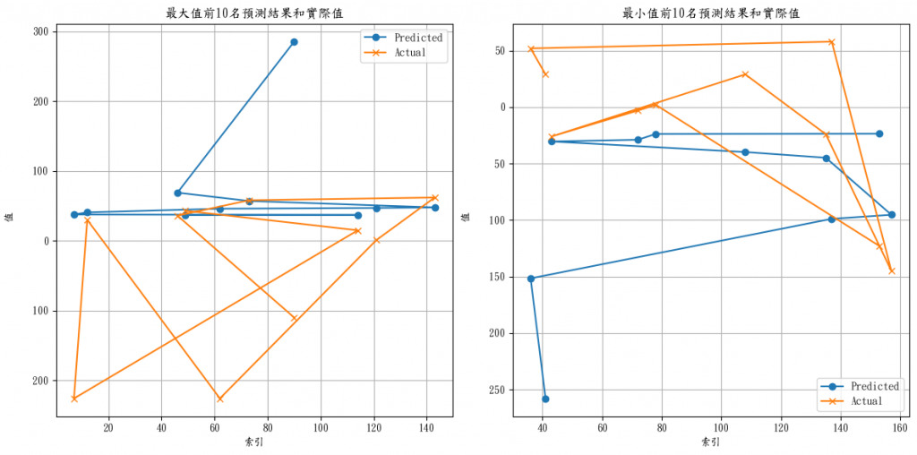
有些人習慣直接看數字，有些人喜歡看圖表，

接著再把買超前10名、賣超前10名的預測值、實際值，視覺化成圖表

plt.figure(figsize=(12, 6))

plt.subplot(1, 2, 1)
plt.plot(top_10_max['預測值'], label='Predicted', marker='o')
plt.plot(top_10_max['實際值'], label='Actual', marker='x')
plt.title('最大值前10名預測結果和實際值')
plt.xlabel('索引')
plt.ylabel('值')
plt.legend()
plt.grid(True)

plt.subplot(1, 2, 2)
plt.plot(top_10_min['預測值'], label='Predicted', marker='o')
plt.plot(top_10_min['實際值'], label='Actual', marker='x')
plt.title('最小值前10名預測結果和實際值')
plt.xlabel('索引')
plt.ylabel('值')
plt.legend()
plt.grid(True)

# 把買超、賣超兩張合併在一起
plt.tight_layout()
plt.show()