四顧模型迎來的春天，時空資料的ConvLSTM模型訓練成功!

2024 iThome 鐵人賽

DAY 22

Python

時空序列分析-關鍵籌碼分析系列第 22 篇

16th鐵人賽 day22 時空序列分析-關鍵籌碼分析

decent_bo_yan

2024-08-22 13:50:10

153 瀏覽

分享至

分析在昨天和前天的模型當中，預測結果出現`NaN`，

可能是這幾個原因造成的:

資料一次顯示太多，圖表無法正常顯示，可以只列出部分先觀察。

資料中可能有NaN值、無效值，沒有清理乾淨，導致模型訓練出問題。

模型架構有問題，可能是資料架構還是不符合模型。

資料前處理有問題，資料標準化、正規化沒有處理好。

針對一、二的問題，

為了驗證昨天模型的值到底是太小看不出來，還是都是NaN值，
避免是將資料全部印出太密集看不見的問題，只顯示前20筆預測結果，可以這麼寫:

# 檢查預測值中，是否有NaN值
if np.isnan(predictions).any():
    print("Predictions contain NaN values.")
else:
    print("No NaN values in predictions.")

# 只顯示前20筆預測值
plt.plot(predictions[:20], label='Predicted')
plt.plot(y_test[:20], label='Actual')
plt.legend()
plt.show()

接著針對三、四的問題，

就直接把整段程式碼檢查一遍，審視哪一個環節出問題。

import pandas as pd
import numpy as np
from keras.models import Sequential
from keras.layers import ConvLSTM2D, Flatten, Dense
from tensorflow.keras.optimizers import Adam
from sklearn.model_selection import train_test_split
from PIL import Image
import matplotlib.pyplot as plt
from sklearn.metrics import mean_squared_error

# 讀取保存的圖像並轉換為資料矩陣
image = Image.open('broker_locations.png')
image = image.convert('L')  # 轉為灰度圖像
image = image.resize((100, 100), Image.Resampling.LANCZOS)  # 缩小圖像

data_matrix = np.array(image).astype(np.float32)
channels = 1

這邊添加一個步驟，

除了要檢查輸入資料有NaN以外，再用平均值去取代這些無效值

# Excel讀取進來
dataOri = pd.read_excel('Merged_to_train_ALL_trans_New.xlsx')
df = pd.DataFrame(dataOri)

# Convert columns to numeric, errors='coerce' will convert non-convertible values to NaN
for col in df.columns[1:]:
    df[col] = pd.to_numeric(df[col], errors='coerce')

# 設置券商代碼為索引
df.set_index('券商代碼', inplace=True)

# 用資料表中的數值計算出來的平均值，來取代NaN值
df.fillna(df.mean(), inplace=True)
df#print(df)

2024/05/13 2024/05/14 2024/05/15 2024/05/16
券商代碼
1020 18 -19.0 3.0 37.0
1021 -79 -17.0 -27.0 15.0
1022 -18 -4.0 -2.0 17.0
1023 26 4.0 -7.0 38.0
1024 3 -30.0 -8.0 8.0
... ... ... ... ...
9A9j -4 6.0 39.0 -47.0
9A9q -5 8.0 -1.0 -26.0
9A9r 0 251.0 -21.0 -226.0
9A9s 0 -11.0 -4.0 8.0
9A9x -4 -27.0 -20.0 -15.0
811 rows × 4 columns

# 創建時間序列資料
def create_sequences(data, time_steps=3):
    X, y = [], []
    for i in range(len(data) - time_steps):
        X.append(data[i:i+time_steps, :])  # Use all columns
        y.append(data[i+time_steps, -1])     # Use the last column as the target
    return np.array(X), np.array(y)

data = df.values

# 創建輸入和輸出資料
X, y = create_sequences(data, time_steps=3)

# 切割資料，在資料合併前就先以8:2切割成訓練集和測試集
X_train, X_test, y_train, y_test = train_test_split(X, y, test_size=0.2, random_state=1024)

print("OK!")

OK!

(把弟兄們清理掉了，世界和平)

# 建立圖像資料
width = data_matrix.shape[1]
height = data_matrix.shape[0]

# 將時間序列資料擴展為與圖像資料相同的形狀
def expand_data(X, width, height):
    X_expanded = np.repeat(X[:, :, np.newaxis, np.newaxis, :], width, axis=2)
    X_expanded = np.repeat(X_expanded, height, axis=3)
    return X_expanded

X_train_expanded = expand_data(X_train, width, height)
X_test_expanded = expand_data(X_test, width, height)

image_data_train = np.tile(data_matrix[np.newaxis, np.newaxis, :, :, np.newaxis], (X_train.shape[0], X_train.shape[1], 1, 1, 1))
image_data_test = np.tile(data_matrix[np.newaxis, np.newaxis, :, :, np.newaxis], (X_test.shape[0], X_test.shape[1], 1, 1, 1))

# 合併時間序列資料和圖像資料
combined_data_train = np.concatenate((X_train_expanded, image_data_train), axis=-1)
combined_data_test = np.concatenate((X_test_expanded, image_data_test), axis=-1)

# 檢查合併後的形狀
print("Combined train data shape:", combined_data_train.shape)
print("Combined test data shape:", combined_data_test.shape)

Combined train data shape: (646, 3, 100, 100, 5)
Combined test data shape: (162, 3, 100, 100, 5)

模型都沒有動，參數一樣

model = Sequential([
    ConvLSTM2D(filters=64, kernel_size=(1, 1), input_shape=(combined_data_train.shape[1:]), return_sequences=True),
    ConvLSTM2D(filters=32, kernel_size=(1, 1), return_sequences=False),
    Flatten(),
    Dense(50, activation='relu'),
    Dense(1)
])

model.compile(optimizer=Adam(learning_rate=0.001), loss='mse')
model.summary()

# 訓練模型
history = model.fit(combined_data_train, y_train, epochs=50, batch_size=32, validation_split=0.1)

Model: "sequential_6"
┃ Layer (type) ┃ Output Shape ┃ Param # ┃
│ conv_lstm2d_12 (ConvLSTM2D) │ (None, 3, 100, 100, 64)│ 17,920 │
│ conv_lstm2d_13 (ConvLSTM2D) │ (None, 100, 100, 32) │ 12,416 │
│ flatten_6 (Flatten) │ (None, 320000) │ 0 │
│ dense_10 (Dense) │ (None, 50) │ 16,000,050 │
│ dense_11 (Dense) │ (None, 1) │ 51 │

Total params: 16,030,437 (61.15 MB)
Trainable params: 16,030,437 (61.15 MB)
Non-trainable params: 0 (0.00 B)

Epoch 1/50
19/19 ━━━━━━━━━━━━━━━━━━━━ 46s 2s/step - loss: 10514.1367 - val_loss: 14555.1826
Epoch 2/50
19/19 ━━━━━━━━━━━━━━━━━━━━ 37s 2s/step - loss: 5318.6313 - val_loss: 14719.3291
... ...
Epoch 50/50
19/19 ━━━━━━━━━━━━━━━━━━━━ 27s 1s/step - loss: 4230.6987 - val_loss: 15423.0039
WARNING:tensorflow:5 out of the last 33 calls to <function TensorFlowTrainer.make_predict_function..one_step_on_data_distributed at 0x000001A8020E7C70> triggered tf.function retracing. Tracing is expensive and the excessive number of tracings could be due to (1) creating @tf.function repeatedly in a loop, (2) passing tensors with different shapes, (3) passing Python objects instead of tensors. For (1), please define your @tf.function outside of the loop. For (2), @tf.function has reduce_retracing=True option that can avoid unnecessary retracing. For (3), please refer to https://www.tensorflow.org/guide/function#controlling_retracing and https://www.tensorflow.org/api_docs/python/tf/function for more details.
6/6 ━━━━━━━━━━━━━━━━━━━━ 4s 534ms/step

發現了什麼!
有東西出來啦~ (賀 (灑花

雖然那個loss差得有點多...@@ 結果感覺就是不太優，但是先求有再求好!!

包括警告訊息@@
了解了一下，好像是因為function會一直在for迴圈創建，
不處理也是影響不大..，要擔心可能會不小心訓練到掛掉(記憶體被吃光

預測的時候，把前面提到的檢查的程式碼也加進來

# 預測一下
predictions = model.predict(combined_data_test)

# 檢查預測值中，是否有NaN值
if np.isnan(predictions).any():
    print("Predictions contain NaN values.")
else:
    print("No NaN values in predictions.")

# 只顯示前20筆預測值
plt.plot(predictions[:20], label='Predicted')
plt.plot(y_test[:20], label='Actual')
plt.legend()
plt.show() #畫圖 視覺化

No NaN values in predictions.

C:\Users\user\AppData\Roaming\Python\Python310\site-packages\IPython\core\pylabtools.py:152: UserWarning: Glyph 8722 (\N{MINUS SIGN}) missing from current font.
fig.canvas.print_figure(bytes_io, **kw)
有時候這種警告訊息可以看一看就好，影響不大。

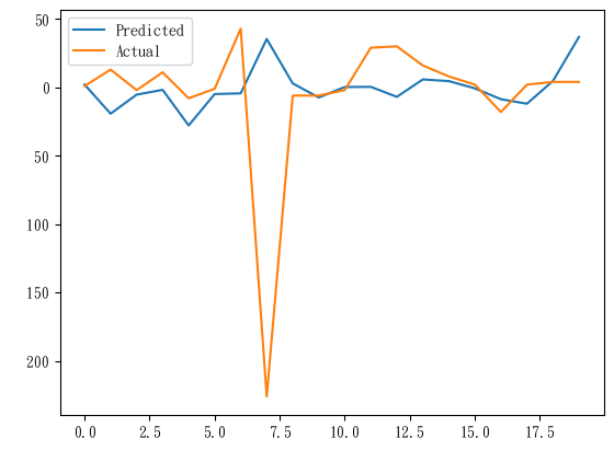
圖還蠻明顯而且看起來有點樣子，
不過軸上沒有標記，要看一下資料才知道數字是甚麼意思。

接著評估一下模型，用`MSE`(均方差)來評估

# 用 MSE 評估模型
mse = mean_squared_error(y_test, predictions)
print("Mean Squared Error:", mse)

Mean Squared Error: 5890.684962306292

MSE本質意義上是指`實際值和預測值之間差的平方和取平均`。

誤差這回事呢，當然預測值離實際值越近越好，所以誤差越小越好...

想了解各種評估方式，可以看[2]這篇文章。
看到這誤差(掩面

先把模型存起來好了..

### 儲存模型
import joblib
# 儲存模型至指定路徑
joblib.dump(model, 'trainModel_0822.joblib')

振作振作，先把預測值和實際值明確印出來看看到底差在哪裡。

印出前20筆的預測結果和實際值

# 印出前20筆預測結果和實際值
print("前20筆預測結果和實際值:")
print("索引\t預測值\t\t實際值")
for i in range(20):
    print(f"{i}\t{predictions[i][0]:.2f}\t\t{y_test[i]:.2f}")

前20筆預測結果和實際值:
索引預測值實際值
0 2.06 1.00
1 -19.23 13.00
2 -5.31 -2.00
3 -1.81 11.00
4 -27.86 -8.00
5 -4.90 -1.00
6 -4.38 43.00
7 35.37 -226.00
8 2.88 -6.00
9 -7.38 -6.00
10 0.26 -2.00
11 0.38 29.00
12 -6.94 30.00
13 5.81 16.00
14 4.58 8.00
15 -0.71 2.00
16 -8.64 -18.00
17 -11.97 2.00
18 4.69 4.00
19 36.89 4.00

再把這個值視覺化得更清楚一點(也加入Label)

# 視覺化前20筆預測結果和實際值
plt.figure(figsize=(10, 6))
plt.plot(predictions[:20], label='Predicted', marker='o')
plt.plot(y_test[:20], label='Actual', marker='x')
plt.title('前20名預測結果和實際值')
plt.xlabel('索引')
plt.ylabel('值')
plt.legend()
plt.grid(True)
plt.show()

C:\Users\user\AppData\Roaming\Python\Python310\site-packages\IPython\core\pylabtools.py:152: UserWarning: Glyph 8722 (\N{MINUS SIGN}) missing from current font.
fig.canvas.print_figure(bytes_io, **kw)

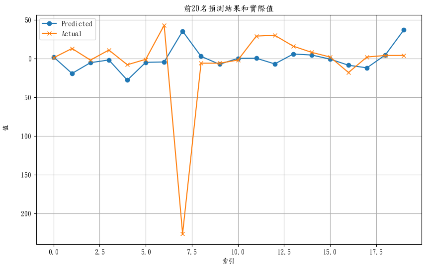
這張圖看起來結果還蠻不錯的阿(只是有一個點就特別奇怪這樣)