至今我們學習的 VGG、ResNet 等模型,它們的設計目標都是追求極致的準確率。然而,這些模型龐大的參數數量和巨大的計算量,使得它們很難被部署到手機、無人機、智慧眼鏡、物聯網等計算資源和電力都極其有限的邊緣設備 (edge devices) 上。因此輕量級網路成為一個重要的研究方向:如何在保持性能的同時,讓 CNN 模型變得更小。
在了解 MobileNet 的解決方案之前,先來分析一下問題的根源:標準的卷積操作,計算成本究竟有多高?
假設我們有一個輸入特徵圖,尺寸為 H × W × C_in(高 × 寬 × 輸入通道數),我們想用 N 個 K × K 大小的卷積核,來生成一個 H × W × C_out 的輸出特徵圖(假設 C_out = N)。
對於輸出特徵圖上的每一個像素點,我們都需要進行一次 K × K × C_in 次乘法運算,而整個輸出特徵圖共有 H × W × C_out 個像素點。
因此,一個標準卷積層的總計算成本約為:
可以看到,計算成本與輸入通道數 C_in 和輸出通道數 C_out 的乘積成正比。當網路很深,通道數很多時(例如 256, 512),這個計算成本會變得非常巨大。
MobileNet 使用了深度可分離卷積 (depthwise separable convolution) 來取代標準卷積,將標準卷積分為兩步
逐深度卷積:只負責空間濾波,為輸入的每一個通道都分配單獨的 K×K 卷積核。假設輸入是 H×W×C_in,那麼經過這一步,會得到一個同樣是 H×W×C_in 的輸出,計算成本為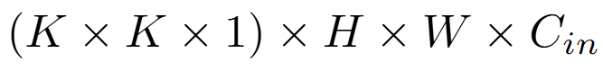
逐點卷積:接在逐深度卷積後,等同於大小為 1×1 的標準卷積。會用 C_out 個 1×1×C_in 大小的卷積核來對第一步的輸出進行卷積。計算成本為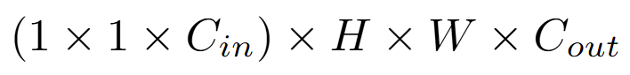
因此總成本為
與標準卷積的成本比率為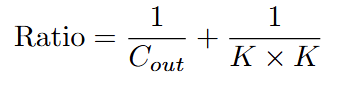
假設我們使用常見的 3x3 卷積核時 (K=3),這個比率約為 1/C_out + 1/9。當輸出通道數 C_out 很大時,這個比率趨近於 1/9。
改進版的 MobileNetV2 則又引入了兩個改進
倒置殘差結構 (inverted residuals): ResNet 中的殘差塊是「寬 -> 窄 -> 寬」的結構,即先用 1×1 卷積降維,再做 3×3 卷積,最後再用 1×1 卷積升維。MobileNetV2 發現,在低維空間中做卷積,會損失太多資訊。因此,它反其道而行之,採用了「窄 -> 寬 -> 窄」的結構:先用 1×1 卷積升維,然後在更寬的特徵空間中進行 3×3 的深度卷積,最後再用 1×1 卷積降維回來。並且,它的捷徑連接是連在兩端的低維「瓶頸層」之間。
線性瓶頸 (linear bottlenecks):團隊還發現,如果在降維後的低維特徵上使用 ReLU 激勵函數,會破壞很多有用的資訊。因此,在倒置殘差結構的最後一個 1x1 卷積層(即降維層)之後,不再使用 ReLU,而是直接進行線性輸出。
import torch
import torchvision.models as models
import time
from ptflops import get_model_complexity_info

# --- 1. 載入模型結構 ---
resnet50 = models.resnet50(pretrained=False)
mobilenet_v2 = models.mobilenet_v2(pretrained=False)

# --- 2. 比較模型大小與參數數量 ---
def count_parameters(model, model_name):
    params = sum(p.numel() for p in model.parameters() if p.requires_grad)
    print(f"{model_name} 的可訓練參數數量: {params / 1_000_000:.2f} M")

count_parameters(resnet50, "ResNet-50")
count_parameters(mobilenet_v2, "MobileNetV2")

# --- 3. 比較計算量 (FLOPs) ---
# FLOPs (Floating Point Operations) 是衡量模型計算複雜度的常用指標
# 檢查是否有CUDA可用,如果沒有則使用CPU
if torch.cuda.is_available():
    with torch.cuda.device(0):
        macs_resnet, params_resnet = get_model_complexity_info(resnet50, (3, 224, 224), as_strings=True, print_per_layer_stat=False, verbose=True)
        macs_mobilenet, params_mobilenet = get_model_complexity_info(mobilenet_v2, (3, 224, 224), as_strings=True, print_per_layer_stat=False, verbose=True)
else:
    macs_resnet, params_resnet = get_model_complexity_info(resnet50, (3, 224, 224), as_strings=True, print_per_layer_stat=False, verbose=True)
    macs_mobilenet, params_mobilenet = get_model_complexity_info(mobilenet_v2, (3, 224, 224), as_strings=True, print_per_layer_stat=False, verbose=True)

print(f"ResNet-50     | {params_resnet:<8} | {macs_resnet:<8}")
print(f"MobileNetV2   | {params_mobilenet:<8} | {macs_mobilenet:<8}")


# --- 4. 比較推論速度 ---
device = torch.device("cuda" if torch.cuda.is_available() else "cpu")
print(f"\n將在 {device} 上比較推論速度...")

resnet50.to(device).eval()
mobilenet_v2.to(device).eval()

# 創建一個隨機的輸入張量
dummy_input = torch.randn(1, 3, 224, 224).to(device)
num_iterations = 100

def measure_inference_time(model, model_name):
    # 預熱
    with torch.no_grad():
        for _ in range(10):
            _ = model(dummy_input)

    # 計時
    start_time = time.time()
    with torch.no_grad():
        for _ in range(num_iterations):
            _ = model(dummy_input)
    end_time = time.time()

    avg_time_ms = (end_time - start_time) / num_iterations * 1000
    fps = 1000 / avg_time_ms
    print(f"{model_name} 平均推論時間: {avg_time_ms:.3f} ms/image | FPS: {fps:.2f}")

measure_inference_time(resnet50, "ResNet-50  ")
measure_inference_time(mobilenet_v2, "MobileNetV2")
結果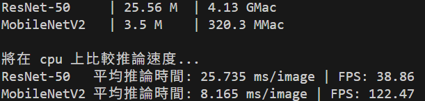


 iThome鐵人賽