【Day 11】資料探索性分析與視覺化

17th鐵人賽

jackietung

2025-09-01 22:54:33

30 瀏覽

分享至

前言

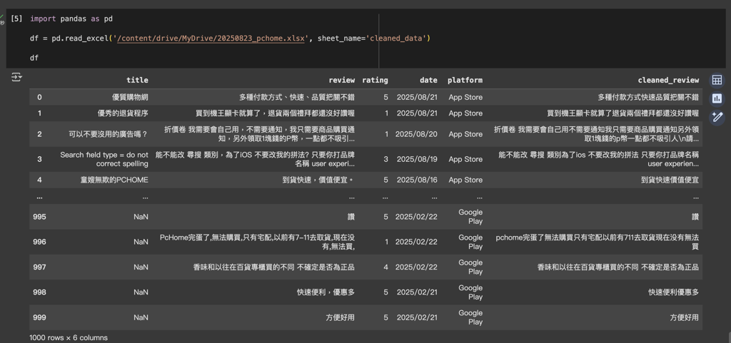
在上一篇文章中，我們已經完成資料集的清理工作。接下來，我們將進行初步的資料探勘，透過視覺化方式分析目前評論的分布狀況，從中獲得初步洞察。

Step 1：讀取清理後的資料

首先，我們從雲端儲存空間讀取之前清理好的資料檔案：

import pandas as pd

# 從指定路徑讀取已清理的資料
df = pd.read_excel('/content/drive/MyDrive/20250823_pchome.xlsx', sheet_name='cleaned_data')
                   
df

Step 2：分析評論的時間分布

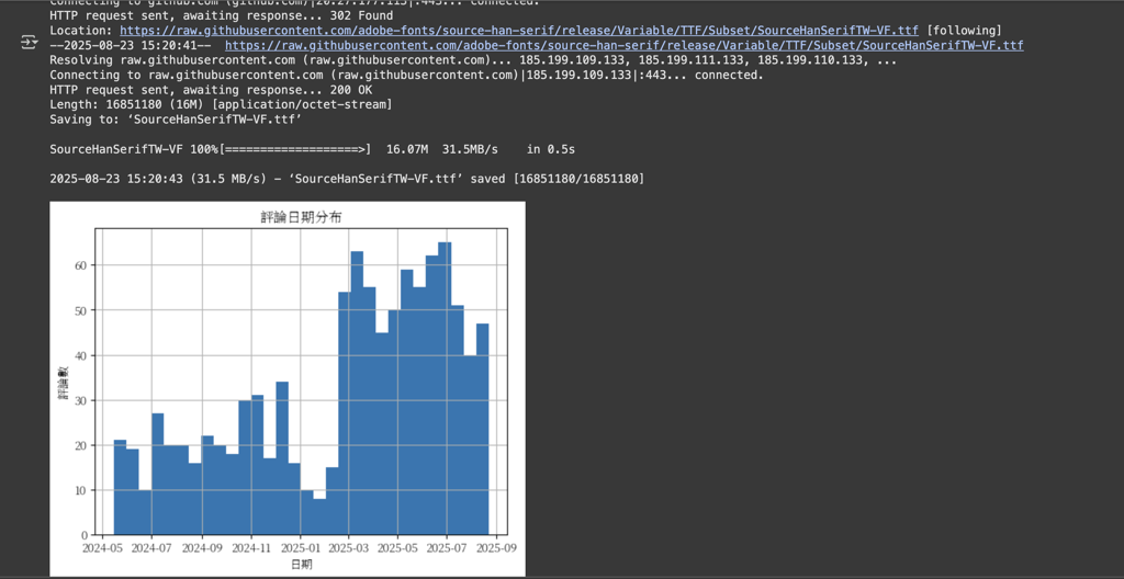
了解評論的時間分布有助於我們辨識評論數的趨勢。首先安裝必要的套件並設定中文字型：

!pip install wordcloud matplotlib -qqq

import matplotlib as mpl
import matplotlib.font_manager as fm
import matplotlib.pyplot as plt

# 下載並設定繁體中文字型
!wget -O SourceHanSerifTW-VF.ttf https://github.com/adobe-fonts/source-han-serif/raw/release/Variable/TTF/Subset/SourceHanSerifTW-VF.ttf
fm.fontManager.addfont('SourceHanSerifTW-VF.ttf')
mpl.rc('font', family='Source Han Serif TW VF')

# 將日期欄位轉換為日期格式並繪製直方圖
df['date'] = pd.to_datetime(df['date'], errors='coerce')
plt.figure(figsize=(10, 6))
df['date'].hist(bins=30)
plt.title('評論日期分布')
plt.xlabel('日期')
plt.ylabel('評論數')
plt.tight_layout()
plt.show()

Step 3：分析評論星等分布

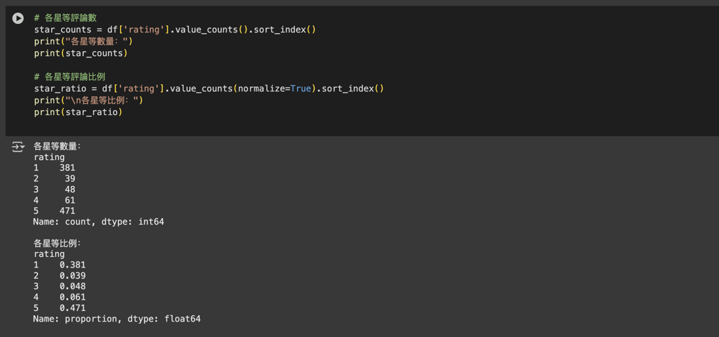
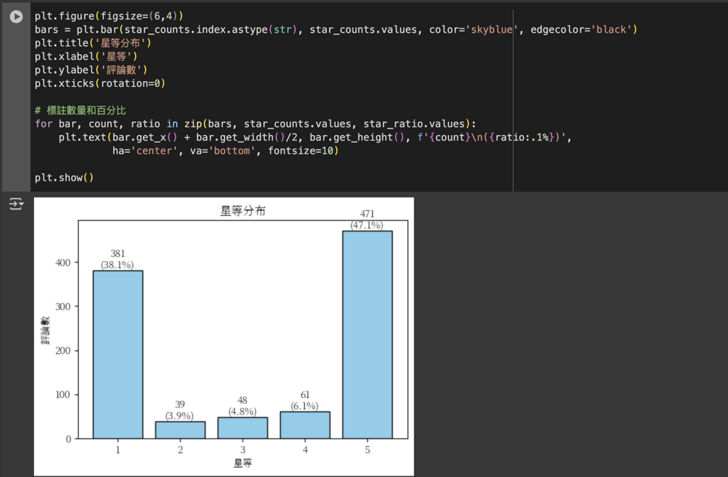
星等分布可以反映用戶對產品或服務的整體滿意度

plt.figure(figsize=(8, 5))
star_counts = df['star'].value_counts().sort_index()
star_ratio = star_counts / star_counts.sum()

bars = plt.bar(star_counts.index.astype(str), star_counts.values, color='skyblue', edgecolor='black')
plt.title('評論星等分布')
plt.xlabel('星等')
plt.ylabel('評論數')
plt.xticks(rotation=0)

# 在每個柱狀圖上標註數量和百分比
for bar, count, ratio in zip(bars, star_counts.values, star_ratio.values):
    plt.text(bar.get_x() + bar.get_width()/2, bar.get_height(), 
             f'{count}\n({ratio:.1%})', 
             ha='center', va='bottom', fontsize=10)

plt.tight_layout()
plt.show()

Step 4：使用 TF-IDF 進行文字探勘

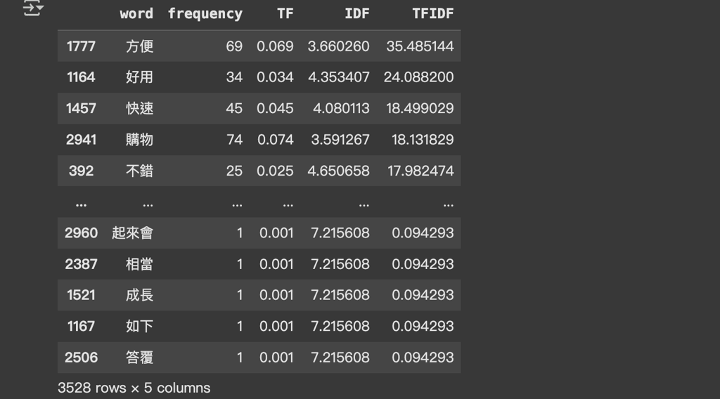
接下來，我們使用 TF-IDF (Term Frequency-Inverse Document Frequency) 技術來辨識評論中的關鍵詞彙。

import jieba
from sklearn.feature_extraction.text import TfidfVectorizer

# 定義停用詞列表
stopwords = ["一直", "無法", "沒有", "app", "App", "APP",
    "就是", "但是", "而且", "所以", "因為", "這個", "這樣", "到底",
    "非常", "使用", "還有", "只有", "收到", "顯示", "通知",
    "直接", "什麼", "處理", "good", "真的", "結果"]

# 定義分詞與過濾停用詞的函式
def tokenize_review(review, stopwords):
    """
    分詞並過濾停用詞
    :param review: 單一文本
    :param stopwords: 停用詞集合
    :return: 過濾停用詞後的分詞結果，格式為空格分隔的字串
    """
    if pd.isna(review):  # 若欄位為 NaN，回傳空字串
        return ""
    words = jieba.lcut(review, cut_all=False)  # 精確模式分詞
    return " ".join([word for word in words if word not in stopwords])  # 過濾停用詞

def tokenize_reviews(df, review_col, stopwords):
    result_df = df.copy()
    result_df['review_tokenized'] = result_df[review_col].apply(lambda x: tokenize_review(x, stopwords))
    return result_df

def calculate_tfidf(reviews, stopwords):
    # 使用 TF-IDF 向量化文本
    vectorizer = TfidfVectorizer()
    tfidf_matrix = vectorizer.fit_transform(reviews)
    vocab = vectorizer.get_feature_names_out()
    idf_values = vectorizer.idf_

    # 計算詞彙出現次數（TF）和 TF-IDF
    word_count = (tfidf_matrix > 0).sum(axis=0).A1  # 詞出現次數
    tf_values = word_count / len(reviews)  # 平均 TF 值
    tfidf_values = tfidf_matrix.toarray().sum(axis=0)

    # 建立結果 DataFrame
    tfidf_summary_df = pd.DataFrame({
        "word": vocab,
        "frequency": word_count,
        "TF": tf_values,
        "IDF": idf_values,
        "TFIDF": tfidf_values
    })

    return tfidf_summary_df.sort_values(by="TFIDF", ascending=False)

# 處理評論文本
tokenize_df = tokenize_reviews(df, 'review', stopwords)

# 計算 TF-IDF 並顯示結果
tfidf_summary_df = calculate_tfidf(tokenize_df['review_tokenized'], stopwords)
tfidf_summary_df.head(20)  # 顯示前20個關鍵詞

Step 5：生成文字雲視覺化

最後，我們將 TF-IDF 分析的結果轉換為文字雲，抓出用戶所提及的熱度關鍵字有哪些，例如「好用」、「快速」、「便宜」等等。

from wordcloud import WordCloud
import urllib.request
import os

def create_wordcloud(word_df):
    """
    從詞頻DataFrame生成文字雲
    
    Parameters:
    word_df: 包含詞頻的DataFrame，需要有 'word' 和 'frequency' 列
    """
    # 檢查字體文件是否存在
    font_path = 'TaipeiSansTCBeta-Regular.ttf'
    if not os.path.exists(font_path):
        print("下載字體文件...")
        url = "https://drive.google.com/uc?id=1eGAsTN1HBpJAkeVM57_C7ccp7hbgSz3_&export=download"
        urllib.request.urlretrieve(url, font_path)

    # 添加字體
    fm.fontManager.addfont(font_path)
    plt.rc('font', family='Taipei Sans TC Beta')

    # 將DataFrame轉換為字典格式
    word_freq_dict = dict(zip(word_df['word'], word_df['frequency']))

    # 生成文字雲
    wordcloud = WordCloud(
        font_path=font_path,
        width=800,
        height=400,
        background_color='white',
        max_words=100,  # 最多顯示100個詞
        min_font_size=10,
        max_font_size=100
    ).generate_from_frequencies(word_freq_dict)

    # 顯示文字雲
    plt.figure(figsize=(12, 6))
    plt.imshow(wordcloud, interpolation='bilinear')
    plt.axis("off")
    plt.title("評論關鍵詞文字雲", fontsize=16)
    plt.tight_layout(pad=0)
    plt.show()

    return wordcloud

# 生成文字雲
try:
    wordcloud = create_wordcloud(tfidf_summary_df)
except Exception as e:
    print(f"生成文字雲時發生錯誤: {str(e)}")