風格遷移是一種很帥、但其實概念蠻優雅的技術：
把一張圖片的內容，配上另一張圖片的風格，生出一張既保留原始場景、又帶有名畫或特定質感的新圖。想像：把你家的街景照，畫成梵谷、莫內或浮世繪版本。

風格遷移迷人的地方在於，它做的不是「套濾鏡」，而是把圖片拆成兩件事再組回來：內容和風格。傳統濾鏡只是整張圖一起調色加效果，風格遷移則是先從內容圖取出場景結構與物體位置（房子、人、樹在哪），再從風格圖學紋理、筆觸、顏色與光影氛圍，最後生成一張同時滿足「長得像原場景」又「有指定畫風」的新圖片。這是靠 CNN 不同層次的特徵來做到的：淺層負責內容輪廓，深層負責風格特徵，我們不重訓模型，而是借用這些中間層輸出作為描述子。

三、內容損失：生成圖要像「原圖的樣子」

我們希望生成圖的 內容 跟內容圖接近，例如建築位置、人物輪廓還認得出來。

做法是：

1.把內容圖和生成圖都丟進同一個 CNN。

2.在某個中間層（例如 VGG 的 conv4_2）取出 feature map。

3.計算兩者 feature map 的差異（通常是歐氏距離 / MSE）。

4.Content Loss越小，代表生成圖的結構越接近原內容。

在內容部分，我們會把內容圖與生成圖丟進同一個 CNN，選定像 VGG 的 conv4_2 這類中間層作為內容特徵，計算兩者特徵圖的差異（例如用 MSE）當作內容損失（Content Loss）。這個值越小，代表生成圖的結構越接近原圖：房子還在原來的位置、人還認得出來，只是畫風被換成了另一種風格。

關鍵工具：Gram 矩陣（Gram Matrix）

步驟：

1對風格圖，取出多個層的 feature maps（例如 conv1_1, conv2_1, ...）。

2對每個層的 feature map，算出通道與通道之間的相關性 → 得到 Gram 矩陣。

3對生成圖做一樣的事。

4比較兩者 Gram 矩陣的差（MSE）

💻 實作流程 (我使用的是colab 作為練習)

1. 準備環境、圖片與預處理
   首先，我們需要準備內容圖片和風格圖片，並定義將圖片轉換為模型可處理張量（Tensor）的函式。

程式碼：圖片路徑與尺寸設定
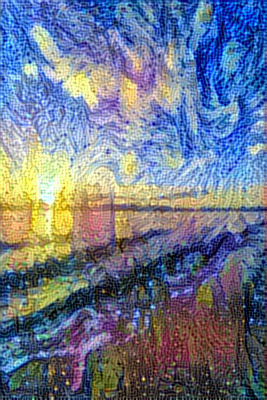
在這個實作中，內容圖片是 picture.jfif，風格圖片是梵谷的《星夜》（starry_night.jpeg）。

from tensorflow import keras
import numpy as np

# 內容圖片與風格圖片路徑
base_image_path='/content/drive/MyDrive/Paint/picture.jfif'
style_reference_image_path='/content/drive/MyDrive/Paint/starry_night.jpeg'

# 定義目標尺寸（將圖片高度固定為 400 像素）
original_width,original_height = keras.utils.load_img(base_image_path).size
img_height = 400
img_width = round(original_width * img_height / original_height)

圖片預處理與後處理
這是確保圖片格式符合 VGG-19 模型輸入要求的重要步驟。

def preprocess_image(image_path):
  # 載入圖片並縮放至目標尺寸
  img = keras.utils. load_img(
      image_path, target_size=(img_height, img_width))
  img= keras.utils.img_to_array(img)
  # 增加批次維度 (batch dimension)
  img= np. expand_dims (img, axis=0)
  # 使用 VGG19 內建的預處理（例如，中心化和 BGR 轉換）
  img= keras.applications.vgg19.preprocess_input(img)
  return img

def deprocess_image(img):
  # 移除批次維度
  img = img.reshape((img_height,img_width,3))
  # 還原 VGG19 預處理時減去的平均值
  img[:,:,0] += 103.939
  img[:,:,1] += 116.779
  img[:,:,2] += 123.68
  # 將 BGR 轉換回 RGB
  img =img[:, :, ::-1]
  # 裁剪像素值到 [0, 255] 範圍並轉換為整數
  img= np.clip(img,0,255).astype("uint8")
  return img

2. 模型載入與特徵提取器
   我們使用預訓練的 VGG-19 模型，但移除頂部的分類層 (include_top=False)，並將其作為特徵提取器。

model = keras.applications.vgg19.VGG19(weights="imagenet",include_top=False)
# 創建一個字典，將層名稱映射到其輸出張量
outputs_dict = dict([(layer.name, layer.output) for layer in model.layers])
# 創建特徵提取器模型：輸入為 VGG19 輸入，輸出為指定層的輸出
feature_extractor = keras.Model(inputs=model.inputs,outputs=outputs_dict)

3. 定義損失函數
   風格遷移的關鍵在於定義三種損失：內容損失、風格損失和總變差損失。

程式碼：內容損失（Content Loss）
內容損失使用內容圖片和生成圖片在 CNN 某個中間層的特徵圖上的歐氏距離。

import tensorflow as tf

def content_loss (base_img, combination_img):
  # 計算特徵圖的平方差之和
  return tf.reduce_sum(tf.square(combination_img - base_img))

風格損失（Style Loss）與 Gram 矩陣
風格特徵由 Gram 矩陣（特徵圖向量之間的相關性）來捕捉。風格損失是兩張圖片的 Gram 矩陣之間的距離。

def gram_matrix(x):
  # 將特徵圖轉換為 (C, H*W) 的矩陣
  x =tf.transpose(x,(2,0,1))
  features = tf. reshape(x,(tf.shape(x)[0], -1))
  # Gram 矩陣 = features 乘以 features 的轉置
  gram = tf.matmul(features,tf.transpose(features))
  return gram

def style_loss(style_img,combination_img):
  S = gram_matrix(style_img)
  C = gram_matrix(combination_img)
  channels = 3
  size = img_height * img_width
  # 風格損失是 Gram 矩陣的平方差之和，並進行歸一化
  return tf.reduce_sum( tf.square(S - C))/(4.0 * (channels **2) * (size ** 2))

總變差損失（Total Variation Loss）
總變差損失是一種**正規化（Regularization）**項，用於鼓勵生成圖片具有空間上的連續性，減少圖片中不自然的噪點。

def total_variation_loss(x):
  # 計算水平方向的像素差平方
  a= tf.square(
    x[:,:img_height - 1,: img_width - 1,:]-x[:,1:,:img_width - 1,:]
  )
  # 計算垂直方向的像素差平方
  b= tf.square(
    x[:,: img_height- 1,: img_width- 1,:]-x[:, : img_height- 1, 1:, :]
  )
  # L1.25 範數
  return tf.reduce_sum(tf.pow(a + b, 1.25))

4. 損失層次與權重配置
   選擇用於提取特徵的層次以及設定各項損失的權重是影響結果風格和內容平衡的關鍵。

style_layer_names = [
    "block1_conv1",
    "block2_conv1",
    "block3_conv1",
    "block4_conv1",
    "block5_conv1",
] # 使用 VGG19 的多個淺層到深層來捕捉風格

content_layer_name = "block5_conv2" # 使用單個深層來捕捉內容

# 權重配置（用於調整內容、風格和噪點的影響程度）
total_variation_weight = 1e-6
style_weight = 1e-6
content_weight = 2.5e-8

總損失計算函式
這個函式負責將所有損失項加權組合起來。

def compute_loss (combination_image, base_image, style_reference_image):
  # 將三個圖片堆疊起來一次性送入模型，以提高效率
  input_tensor = tf.concat(
    [base_image, style_reference_image,combination_image], axis=0
  )
  features = feature_extractor (input_tensor)
  loss = tf.zeros (shape=())

  # 1. 內容損失計算
  layer_features = features[content_layer_name]
  base_image_features = layer_features [0,:,:,:] # 第一個圖（內容圖）的特徵
  combination_features = layer_features [2, :, :, :] # 第三個圖（生成圖）的特徵
  loss = loss + content_weight * content_loss(
    base_image_features, combination_features
  )

  # 2. 風格損失計算（遍歷所有風格層）
  for layer_name in style_layer_names:
    layer_features = features [layer_name]
    style_reference_features = layer_features [1, :, :,:] # 第二個圖（風格圖）的特徵
    combination_features = layer_features [2, :, :,:]
    style_loss_value = style_loss(
      style_reference_features, combination_features)
    # 將總風格權重平均分配給每個風格層
    loss += (style_weight / len(style_layer_names)) * style_loss_value

  # 3. 總變差損失
  loss += total_variation_weight * total_variation_loss(combination_image)
  return loss

5. 優化與迭代迴圈
   優化的目標是直接調整**生成圖片（Combination Image）**的像素值，使其總損失最小化。梯度計算與優化器設定使用 tf.GradientTape 計算損失對生成圖片的梯度，並使用帶有衰減的 SGD 優化器進行更新。

@tf.function
def compute_loss_and_grads(combination_image, base_image, style_reference_image) :
  with tf.GradientTape() as tape:
    # 紀錄計算過程，以便計算梯度
    loss = compute_loss (combination_image, base_image, style_reference_image)
  # 計算損失對 combination_image 的梯度
  grads = tape.gradient (loss, combination_image)
  return loss, grads

# 設定優化器：帶有指數衰減學習率的 SGD
optimizer = keras. optimizers.SGD(
  keras.optimizers.schedules.ExponentialDecay(
    initial_learning_rate=100.0, decay_steps=100, decay_rate=0.96
  )
)

程式碼：主迭代迴圈
這是風格遷移的核心過程，圖片的像素值在這裡被逐步優化。

# 準備輸入圖片並將生成圖片初始化為內容圖片
base_image = preprocess_image(base_image_path)
style_reference_image = preprocess_image(style_reference_image_path)
# 將生成圖片宣告為 tf.Variable，因為它的值將在訓練中更新
combination_image = tf.Variable(preprocess_image(base_image_path))

iterations = 4000 # 總迭代次數
for i in range(1, iterations + 1):
  print('iterations:{0}'.format(i))
  # 1. 計算當前損失和梯度
  loss, grads = compute_loss_and_grads(
      combination_image, base_image, style_reference_image
  )
  # 2. 應用梯度，更新圖片像素
  optimizer.apply_gradients([(grads, combination_image)])
  
  # 3. 每 100 次迭代保存並顯示進度
  if i%100 == 0:
    print(f"Iteration{i}: loss={loss:.2f}")
    img = deprocess_image(combination_image.numpy())
    fname = f"combination_image_at_iteration_{i}.png"
    keras.utils.save_img(fname, img)

這樣就完成一個小小的實作了