本文將簡單介紹用於邊緣偵測的 Laplacian 算子，並示範如何用 OpenCV 的 Laplacian 對灰階圖片進行邊緣偵測，如下圖所示。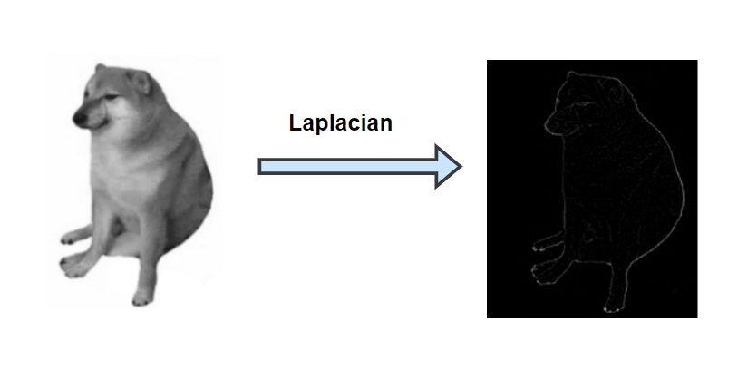

Laplacian 概念:

• 仔細觀察，我們可以發現 edge 附近的像素值會有"劇烈的變化"，所以很自然會跟微積分聯想再一起。

• 可是我們知道灰階圖片是二維陣列，陣列中的每個元素對應為像素的亮度(0-255)，是離散的，連"連續"的概念都沒有，更不用說要用到微積分了，所以我們需要發揮一點想像力，將這些二微陣列的圖片視為某個良好(Differentiability class，C^k class)曲面(surface)上的樣本點(samples)， 便可透過有限差分法(Finite Difference Method)，去對像素值的劇烈變化做類似的微分估計。

• 同理，我們可以得到二階偏微分 f_xx， f_yy 並將其和 3X3 的 Kernel 做連結。

• 但通過那些灰階圖片樣本點的曲面照理來說有無窮多個，我們只是假設曲面有很好的性質(例如可以微分)，實際上我們也無從得知那是極大值或是極小值或是鞍點或者都不是，但我們前面說過了，edge 附近的像素值會有"劇烈的變化"。此時我們再發揮想像力，想像通過樣本點的曲面是某塊地型，則邊緣附近可以看成是平坦的地形銜接陡峭的峭壁，因此邊緣附近的的散度可能會較大。

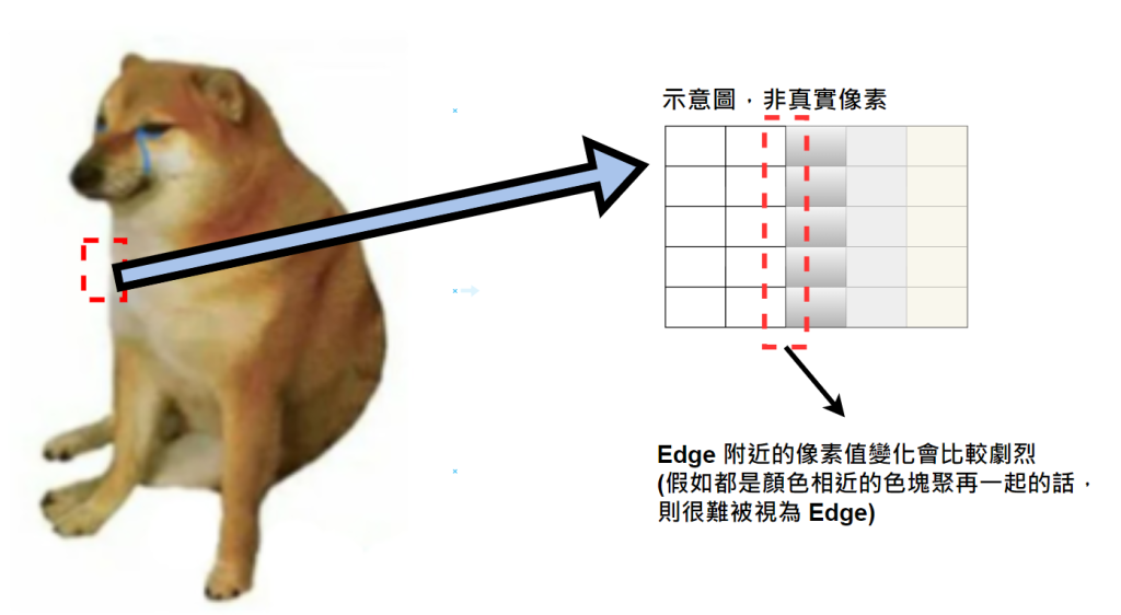
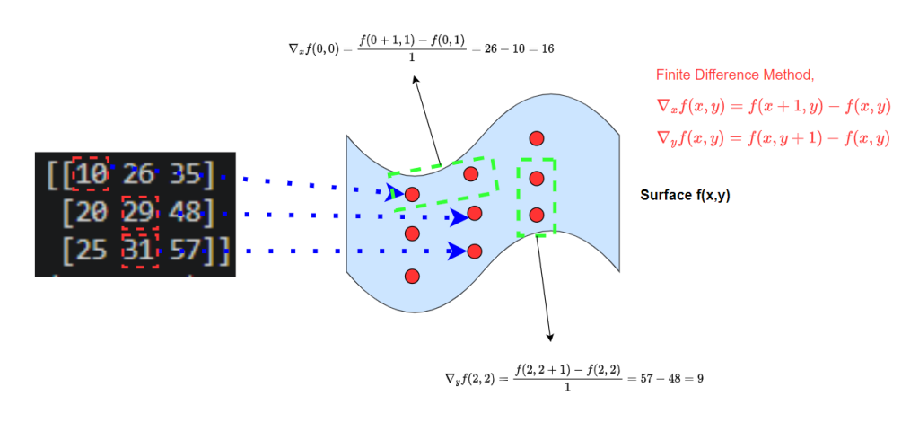
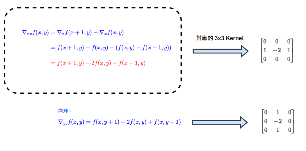
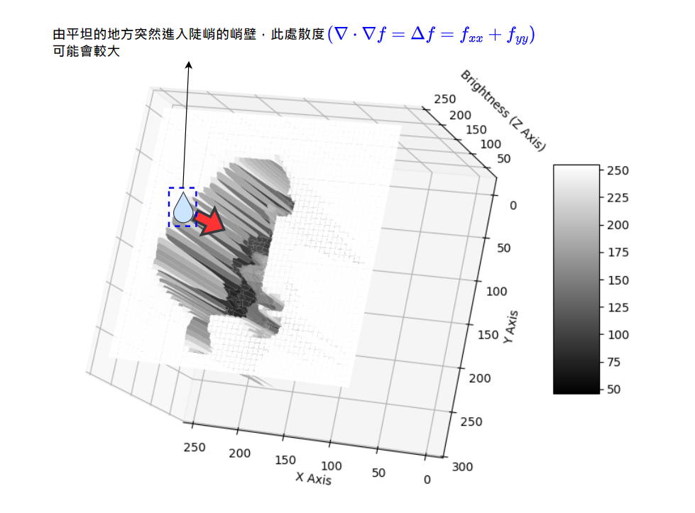
(圖片由下方的 Python 程式碼產生)

import cv2
import numpy as np
import matplotlib.pyplot as plt

dog_pic = '../images/dog.png'  # 圖片位址

dog_img = cv2.imread(dog_pic) 
dog_img_gray = cv2.cvtColor(dog_img, cv2.COLOR_BGR2GRAY)

height, width = dog_img_gray.shape

X = np.arange(0, width, 1)
Y = np.arange(0, height, 1)
X, Y = np.meshgrid(X, Y)
 
# 繪製曲面
fig = plt.figure(figsize=(10, 7))
ax = fig.add_subplot(projection='3d')

surf = ax.plot_surface(
    X, Y, dog_img_gray,  cmap='gray'
)

# 加入色彩條
fig.colorbar(surf, shrink=0.5, aspect=5)

ax.set_xlabel('X Axis')
ax.set_ylabel('Y Axis')
ax.set_zlabel('Brightness (Z Axis)')

plt.show()

• 而剛剛我們也將 f_xx 和 f_yy 和對應的 3x3 kernel 做關聯了，所以很直覺的將兩個 Kernel 相加，可以得到 Laplacian Kernel ➡️ 使用 Laplacian Kernel 去對灰階圖片做捲積後，得到的二維陣列內的每個元素代表該像素的散度大小，也就是說，邊緣可能會發生在那些散度大的地方!!!

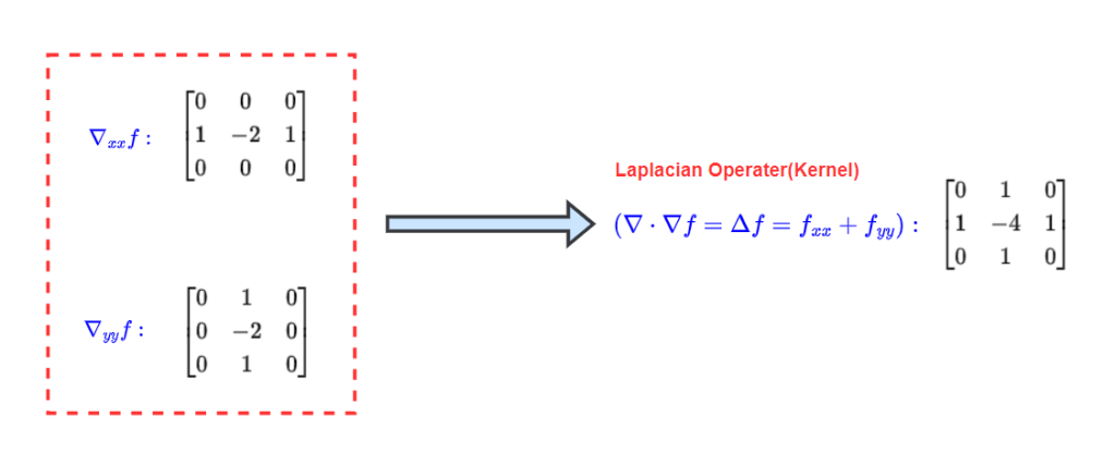
底下為使用Laplacian Kernel 去對灰階圖片做捲積的程式碼:

程式碼(Python):

import cv2
import numpy as np
import matplotlib.pyplot as plt

dog_pic = '../images/dog.png' # 圖片位址

dog_img = cv2.imread(dog_pic) 
dog_img_gray = cv2.cvtColor(dog_img, cv2.COLOR_BGR2GRAY) 

laplacian_kernel = np.array([[0, 1, 0],
                             [1, -4, 1],
                             [0, 1, 0]])

# 也可將等號右邊替代成 cv2.Laplacian(dog_img_gray, -1, 3)
laplacian_img = cv2.filter2D(src=dog_img_gray, ddepth = -1, kernel = laplacian_kernel)

cv2.imshow('before vs after laplacian', np.hstack([dog_img_gray, laplacian_img]))
 
cv2.waitKey()
cv2.destroyAllWindows()

執行結果: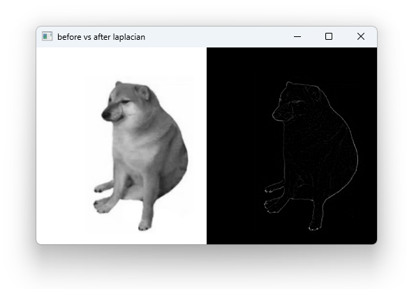

可以發現捲積完的二維矩陣，散度較大的地方(白色線條)和邊緣有蠻大的關連性。

Note:

• 進行邊緣偵測時，主要關注的是影像亮度的變化，因此通常會將彩色圖片轉成灰階，而最常見的 rgb 轉灰階公式為:gray = 0.299r + 0.587g + 0.114b，其中 rgb 各系數的權重是根據人眼對不同顏色的敏感程度所訂的。

以上為筆者對 Laplacian 的理解，數學部分可能沒那麼嚴謹，筆記內容如有錯誤竟請多多包容，謝謝~