
上一篇把一個 Transformer Layer 拆成 GEMM、elementwise、reduction 和 data movement。
但同一個 Layer,在 LLM inference 裡其實會跑出兩種完全不同的硬體行為:
Prefill:一次處理整段 Prompt
Decode:每一步只產生一個新 Token
模型權重沒有變,operator 也沒有變。真正改變的是 tensor shape。
以下是在一張閒置的 RTX 6000 Ada 上,使用 Llama-3.2-1B、bf16、batch 1、context length 2048 的測量結果:
| Prefill | Decode | |
|---|---|---|
| Linear Layer 輸入 | [2048, d] |
[1, d] |
| Projection arithmetic intensity | 768 | 1 |
| Attention arithmetic intensity | 819 | 4 |
| Roofline 區域 | Compute-bound | Memory-bound |
| SM Active | 89.9% | 17.0% |
| Tensor Active | 64.1% | 0.1% |
| GPU Clock | 1015 MHz | 2342 MHz |
這兩欄不只是「工作量比較大」和「工作量比較小」。
Prefill 和 Decode 落在 Roofline 的兩側,受到不同的硬體上限限制。
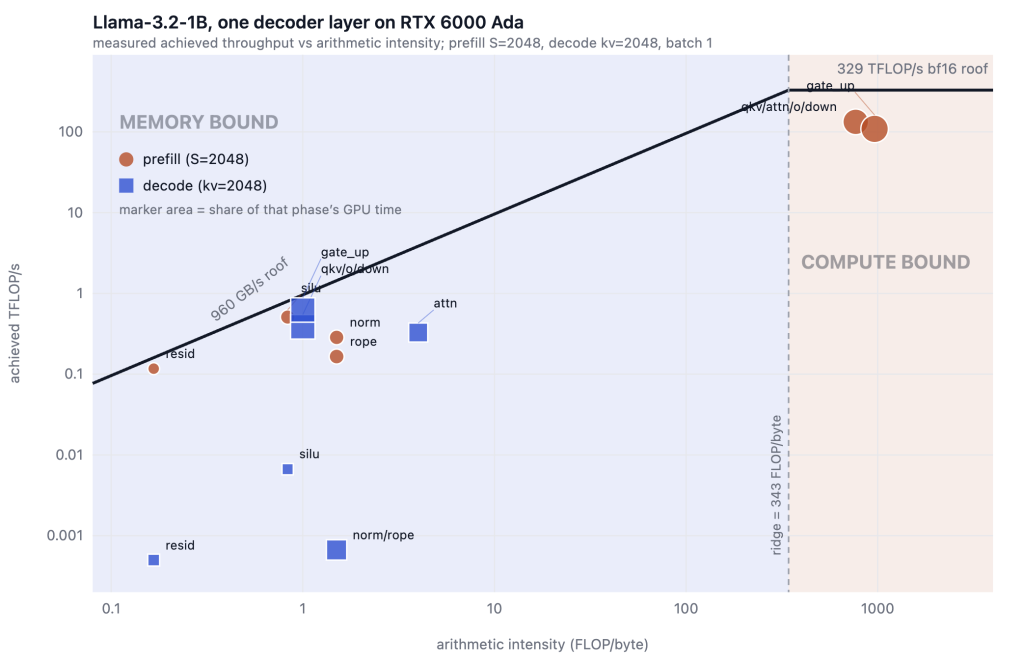
圖中的橘色圓點是 prefill,藍色方塊是 decode;marker 面積代表該操作佔該階段 GPU time 的比例。Prefill 的主要 GEMMs 位於 ridge point 右側,decode operations 則集中在左側的 memory-bound 區域。
Prefill 會把整段 prompt 一次送進模型。
當 sequence length 是 2048 時,Linear Layer 看到的 GEMM 類似:
[2048, d] × [d, N]
同一份權重可以被 2048 個 token 重複使用,因此搬進 GPU 的每個 byte 可以換到很多次運算。
這就是高 arithmetic intensity。
在這次測量中,projection 的 arithmetic intensity 是 768 FLOP/byte,高於這張卡約 343 FLOP/byte 的 ridge point,因此落在 compute-bound 區域。
GPU metrics 也符合這個結果:89.9% 的 SM 處於 active,Tensor Core activity 達到 64.1%。
Clock 反而降到 1015 MHz,是因為密集的 bf16 matrix multiplication 讓這張 300 W GPU 接近 power limit。這個 clock 數字具有硬體特性,但它和高 Tensor Active 一起說明:prefill 真的在大量計算。
Decode 時,前面的 tokens 已經存進 KV Cache,每一步只需要處理最新的一個 token。
Projection 的 shape 於是變成:
[1, d] × [d, N]
矩陣權重仍然要讀取一次,但只服務一個 token。GEMM 退化成接近 GEMV 的工作,幾乎沒有 weight reuse。
對 bf16、batch 1 的 decode projection,可以粗略得到:
Arithmetic Intensity ≈ Batch Size ≈ 1 FLOP/byte
相對於 343 FLOP/byte 的 ridge point,這顯然落在 memory-bound 區域。
實測也看到 SM Active 只有 17.0%,Tensor Active 更只剩 0.1%。GPU 並不是算不動,而是大部分時間沒有足夠的計算可以餵給 Tensor Core。
這時 clock 可以維持在 2342 MHz,但更高的 clock 也無法解決問題:decode 更需要 memory bandwidth,而不是更多 FLOPs。
Projection 要反覆讀取模型權重;attention 則要讀取先前累積的 KV Cache。
對這個使用 GQA 4× 的模型,decode attention 的 arithmetic intensity 約為:
AI = 2 × GQA ratio / bytes per element
   = 2 × 4 / 2
   = 4 FLOP/byte
有趣的是,batch size 和 context length 在這個式子裡會互相消掉。
增加 batch 可以提高 projection 的 weight reuse,卻不會讓每條 sequence 共用彼此的 KV Cache。因此 projection 可能隨 batching 逐漸靠近 compute-bound,decode attention 仍然留在 memory-bound。
這也是 MQA、GQA、KV quantization 和 prefix sharing 都在想辦法減少 KV traffic 的原因。
上一篇看到,一個 Layer 在 PyTorch SDPA 下仍然會展開成 43 個 kernels。
Prefill 時,每個大型 GEMM 可以跑很久,CPU 發出下一個 kernel 的時間不明顯。
Decode 時,每個 kernel 只做很少的工作,GPU 反而可能跑完後等待 CPU 繼續 enqueue。
這可以用 CUDA Graph 做一個很乾淨的對照:
| vLLM | Prefill | Decode / token |
|---|---|---|
| Eager launches | 30.74 ms | 7.982 ms |
| CUDA Graph replay | 30.97 ms | 3.432 ms |
兩邊執行相同 kernels、處理相同資料,只差在 kernel launches 是逐一送出,還是從已錄製的 graph replay。
結果是:
Prefill:幾乎沒有差異
Decode:2.33× faster
CUDA Graph 沒有減少 FLOPs,也沒有增加 memory bandwidth。它只是減少 Python、C++ 和 CUDA driver 的 launch overhead。
這個實驗直接說明:decode 不只 memory-bound,也可能 launch-bound。
Llama-3.2-1B 約有 1.24B parameters。使用 bf16 時,模型權重大約是:
1.24B × 2 bytes = 2.47 GB
RTX 6000 Ada 的 bandwidth 約為 960 GB/s。假設每產生一個 token,權重至少要通過 memory bus 一次:
2.47 GB / 960 GB/s = 2.57 ms/token
也就是理想上限約為 388 tokens/s,而且這還沒有計入 KV Cache、activation、scheduling 和任何其他 overhead。
這次 vLLM + CUDA Graph 實測為 3.43 ms/token,也就是 291 tokens/s,已經達到這個簡化 memory floor 的約 75%。
所以如果只讓 Tensor Core 再快一倍,decode latency 也不會跟著快一倍。權重還是要從 memory 搬進來。



 iThome鐵人賽
 看影片追技術