前言

在上一章介紹了Linear Regression和Logistic Regression，而Logistic Regression使用了一層網路層，效果其實算還不錯了，但若要更精準可以嘗試在多加入網路層，效果可能會更好，而這次要介紹的就是將上篇預測數字的程式碼改寫為多層感知器作法。

訓練步驟

1. 輸入x訓練資料。
2. 預測(乘上權重和加上偏權重)。
3. 活化函數(Relu)。
4. 輸出函數(softmax)。
5. 損失函數。
6. 梯度計算。
7. 使用梯度往回修正權重(反向傳播)。
8. 重複2~7。

多層感知器實作邏輯回歸

與上次不同的地方只有預測函數和損失函數。

初始化

• mnist為讀取mnist資料，設置one_hot(假如是3為[0,0,1,0,....])。
• input_x為輸入訓練資料，input_y為訓練結果，784則是mnist每張圖片像素數量。

mnist = input_data.read_data_sets("MNIST/", one_hot=True)
input_x = tf.placeholder(tf.float32, shape=[None, 784], name="input_x")
input_y = tf.placeholder(tf.float32, shape=[None, 10], name="input_y")

神經層函數

參數：x為輸入資料，weights_shape為權重大小。

• 預設權重設置標準差為**He預設權重**。
• weights為權重，biases為偏權重。
• output為矩陣相乘+上偏移結果，活化函數為relu。

def layer(x, weights_shape):
    init = tf.random_normal_initializer(stddev=np.sqrt(2. / weights_shape[0]))
    weights = tf.get_variable(name="weights", shape=weights_shape, initializer=init)
    biases = tf.get_variable(name="biases", shape=biases_shape, initializer=init)
    output = tf.nn.relu(tf.matmul(x, weights) + biases)
    return output

預測函數

參數：x為訓練資料。

• hide1_size、hide2_size為隱藏層的神經元數量，output_size為輸出數量。

def predict(x):
    with tf.variable_scope("hide1_scope"):
        hide1_out = layer(x, [784, hide1_size])

    with tf.variable_scope("hide2_scope"):
        hide2_out = layer(hide1_out, [hide1_size, hide2_size])

    with tf.variable_scope("hide3_scope"):
        output = layer(hide2_out, [hide2_size, output_size])

    return output

損失函數

使用交叉熵誤差函數。
參數：y為預測結果，t為實際值。

• cross為計算輸出函數(softmax)的交叉熵。
• result為計算平均。(計算平均批量誤差)。
• loss_his為寫入scalar值。

def loss(y, t):
    cross = tf.nn.softmax_cross_entropy_with_logits(logits=y, labels=t)
    result = tf.reduce_mean(cross)
    loss_his = tf.summary.scalar("loss", result)

    return result

訓練函數

參數：loss為損失，index為目前訓練次數。

• learning_rate為學習率，使用SGD類別訓練資料，它會自動綁定loss使用tf計算過的公式，並且自動去計算反向傳播(偏微分)。

def train(loss, index):
    return tf.train.GradientDescentOptimizer(learning_rate).minimize(loss, global_step=index)

驗證函數

參數：output為預測，t為實際。

• comparison為取得目前最大值(索引的對應數字)比較資料是否正確，是輸出1反之輸出0。
• y為計算批量平均誤差。
• 將驗證錯誤率資料寫入scalar。

def accuracy(output, t):
    comparison = tf.equal(tf.argmax(output, 1), tf.argmax(t, 1))
    y = tf.reduce_mean(tf.cast(comparison, tf.float32))

    tf.summary.scalar("accuracy error", (1.0 - y))

    return y

訓練資料

• 訓練次數為train_times，time為第N次訓練。
• avg_loss為記錄訓練資料平均loss。
• batch_size為每次訓練的批量訓練次數，total_batch為計算一次要訓練多少筆。
• 使用mnist.train.next_batch依序取得資料並使用train_op訓練，在計算平均loss。
• 依照設置train_step數字來決定顯示訓練資料週期。
• 運行summary_op(tf.summary.merge_all())取得畫圖資料。
• summary_writer(tf.summary.FileWriter)加入上述運行結果。
• 使用accuracy_op運算顯示目前誤差率。

for time in range(train_times):
    avg_loss = 0.
    total_batch = int(mnist.train.num_examples / batch_size)
    for i in range(total_batch):
        minibatch_x, minibatch_y = mnist.train.next_batch(batch_size)
        session.run(train_op, feed_dict={input_x: minibatch_x, input_y: minibatch_y})
        avg_loss += session.run(loss_op, feed_dict={input_x: minibatch_x, input_y: minibatch_y}) / total_batch

    if (time + 1) % train_step == 0:
        summary_str = session.run(summary_op, feed_dict={input_x: mnist.validation.images, input_y: mnist.validation.labels})
        summary_writer.add_summary(summary_str, session.run(index))
        accuracy = session.run(accuracy_op, feed_dict={input_x: mnist.validation.images, input_y: mnist.validation.labels})
        print("train times:", (time + 1),
                        " avg_loss:", avg_loss,
                        " accuracy:", accuracy)

結果

可以看到結果與上篇的92%相比已經進步了5%至97%，準確度提高非常多。

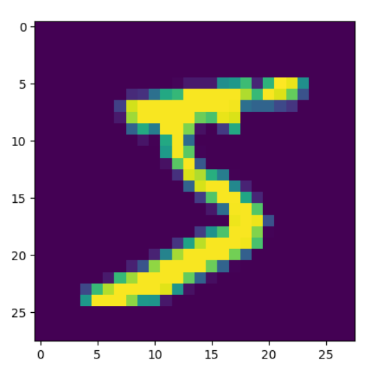
y = session.run(predict_op, feed_dict={input_x:mnist.validation.images[0].reshape(1, 784)})
print("predict : " + str(np.argmax(y)))
print("really: " + str(np.argmax(mnist.validation.labels[0])))
plt.imshow((mnist.validation.images[0].reshape(28, 28)))
plt.show()

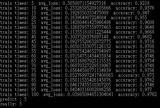
輸出結果。

結語

多層感知器雖然有機會讓數據更佳準確，但也可能會讓準確度更低，因為神經網路內的運算我們不好去控制它最後會產生甚麼，我們只能依照現有的想法和經驗來去調整參數或給予新的公式，若有錯誤地方可在下方留言或私訊謝謝。

參考網址與書籍

[1] https://www.tensorflow.org/api_docs/python/tf
[2] 籃子軒(譯者)（2018）。Deep Learning深度學習基礎｜設計下一代人工智慧演算法。台灣：歐萊禮。