之前在介紹[筆記]深度學習(Deep Learning)-捲積神經網路這篇文章時有提過CNN的原理,而這次使用tensorflow實作,在CNN前會先介紹簡單的影像前置處理。
mnist的資料都是處理過的,而平常假如拿到圖片資料,我們都必須先自己處理,例如灰階、剪裁等等,而tensorflow也有相關函數讓我們使用。
最後這裡範例使用import matplotlib.pyplot as plt的plt.imshow(img)即可展示出來。
1.白化處理。
[2]提到白化處理是先扣掉像素平均值,再將像素的變異量修正到1。
stand_img = session.run(tf.image.per_image_standardization(img)
2.隨機剪裁。
會隨機剪裁大小100*100像素通道為3的圖片。
crop_img = session.run(tf.random_crop(img, size=[100, 100, 3]))
3.隨機上下翻轉。
隨機上或下翻轉圖片。
up_down_img = session.run(tf.image.random_flip_up_down(img))
4.隨機左右翻轉。
隨機左或右翻轉圖片。
left_right_img = session.run(tf.image.random_flip_left_right(img))
5.對角線翻轉。
將圖片對角線翻轉,也就是將轉置圖片軸度。
transpose_img = session.run(tf.image.transpose_image(img))
6.隨機調整亮度。
隨機調整圖片亮度參數max_delta[-max_delta, max_delta]之間,這裡為[-1,1]之間。
brightness_img = session.run(tf.image.random_brightness(img, 1))
7.隨機調整對比。
隨機調整圖片對比,[0.1,0.5]之間。
contrast_img = session.run(tf.image.random_contrast(img, 0.1, 0.5))
8.隨機調整飽和。
隨機調整圖片飽和,[0.1,0.5]之間。
saturation_img = session.run(tf.image.random_saturation(img, 0.1, 0.5))
9.隨機調整色度。
隨機調整圖片色度參數max_delta[-max_delta, max_delta]之間,這裡為[-0.5,0.5]之間。
hue_img = session.run(tf.image.random_hue(img, 0.5))
捲積層為點對點相乘後的總合,而我們稱乘上的板塊為filter,直接看下圖和測試網址即可了解。
捲積後大小以寬為例公式為[(W + (left_pad + right_pad) - CW) / stride + 1],W為原先寬度left_pad和right_pad分別為左右填補大小,CW為捲積寬度,stride為每次移動步伐。以下圖為例,(5 + (0 + 0) - 3) / 1 + 1 = 3,捲積後寬度為3若左右各填補1則捲積後寬度為5。
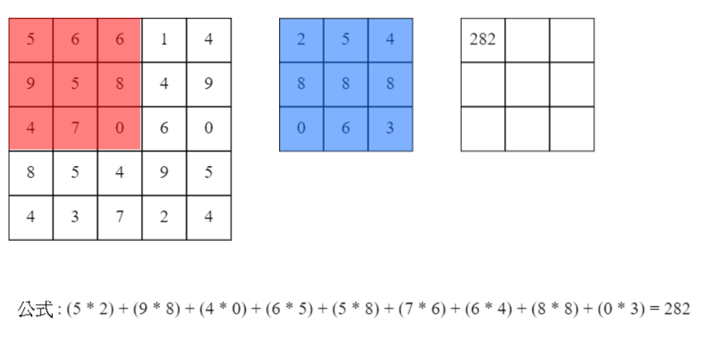
來源:[4]。
池化層則是在區域大小內選出最大的(也有人使用平均等等),直接看下圖和測試網址即可了解。
池化後大小以寬為例公式為[1 + (W - PW) / stride],W為原先寬度,PW為池化寬度,stride為移動大小。以下圖為例,1 + (7 - 2) / 2 = 3,池化後寬度為3(無條件捨去)。
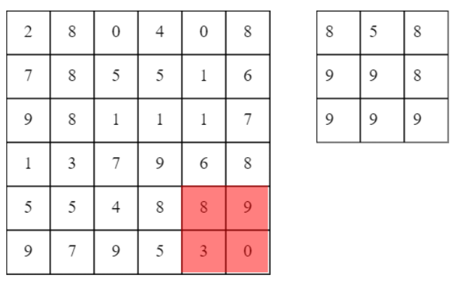
來源:[4]。
這裡使用mnist資料,使用兩個捲積和兩個池化。
1.輸入訓練資料。
2.捲積層。
3.池化層。
4.捲積層。
5.池化層。
6.Dropout(隨機拋棄神經元)。
7.輸出函數(softmax)。
8.損失函數。
9.梯度計算並往回修正權重(反向傳播)。
10.重複2~9至訓練次數。
input_x = tf.placeholder(tf.float32, shape=[None, 784], name="input_x")
input_y = tf.placeholder(tf.float32, shape=[None, 10], name="input_y")
因使用sigmoid所以使用He預設權重([筆記]深度學習(Deep Learning)-神經網路學習的優化),而在這裡可以看到要先計算整理數量,而weight_shape=[資料量, 高度, 寬度, 深度],而批量神經元數量算法為依照深度來轉成二維看待,所以數量大小為為[資料量高度寬度]。
weights為filter權重(四維)[filter數量, 高度, 寬度, 深度],寬度要對應到輸入的(上一層)深度,否則捲積對應數量會錯誤無法計算(算一次就可以知道)。biases_init為filter偏權重(一維),會自動擴展至權重大小。conv_out為捲積函數,strides為每個維度移動的步長。padding為填補模式(SAME為填補0至輸出與原圖大小相同)。conv_add為加上偏權重。output為relu活化函數。def conv2d(input, weight_shape):
size = weight_shape[0] * weight_shape[1] * weight_shape[2]
weights_init = tf.random_normal_initializer(stddev=np.sqrt(2. / size))
biases_init = tf.zeros_initializer()
weights = tf.get_variable(name="weights", shape=weight_shape, initializer=weights_init)
biases = tf.get_variable(name="biases", shape=weight_shape[3], initializer=biases_init)
conv_out = tf.nn.conv2d(input, weights, strides=[1, 1, 1, 1], padding='SAME')
conv_add = tf.nn.bias_add(conv_out, biases)
output = tf.nn.relu(conv_add)
return output
ksize為池化大小,這裡為二維[k高度, k寬度]。strides為步伐,這裡二維步伐[k高度, k寬度],代表不重複走訪。padding為填補模式(SAME為填補0至輸出與原圖大小相同)。def max_pool(input, k=2):
return tf.nn.max_pool(input, ksize=[1, k, k, 1], strides=[1, k, k, 1], padding='SAME')
因使用sigmoid所以使用He預設權重([筆記]深度學習(Deep Learning)-神經網路學習的優化)。
weights為二維權重。biases為一維偏權重,加總會自動擴展。mat_add為輸入乘上權重加上偏權重。output為使用relu活化函數。def layer(x, weights_shape):
init = tf.random_normal_initializer(stddev=np.sqrt(2. / weights_shape[0]))
weights = tf.get_variable(name="weights", shape=weights_shape, initializer=init)
biases = tf.get_variable(name="biases", shape=weights_shape[1], initializer=init)
mat_add = tf.matmul(x, weights) + biases
output = tf.nn.relu(mat_add)
return output
捲積層使用四維,所以會先將mnist轉為四維(8bit單色深度為1),使用兩層捲積+池化,最後轉為二維,使用一層隱藏層(全鏈結層),在經過dropout隨機丟棄神經元(keep_drop為閥值或機率),這裡使用dropout主要可以讓訓練更加穩定,防止每次都訓練一樣的神經元,最後再使用一層隱藏層(全鏈結層)輸出。
conv2d為捲積函數。max_pool為池化函數。layer為一般神經網路(全鏈結層運算)函數。pool2_flat為將每筆資料轉為一維向量。dropout為tensorflow提供的隨機拋棄神經元函數。# [filter size, filter height, filter weight, filter depth]
conv1_size = [5, 5, 1, 32]
conv2_size = [5, 5, 32, 64]
# The new size(7 * 7) before image(28 * 28) used the pooling(2 times) method
hide3_size = [7 * 7 * 64, 1024]
output_size = 10
def predict(x, keep_drop):
x = tf.reshape(x, shape=[-1, 28, 28, 1])
with tf.variable_scope("conv1_scope"):
conv1_out = conv2d(x, conv1_size)
pool1_out = max_pool(conv1_out)
with tf.variable_scope("conv2_scope"):
conv2_out = conv2d(pool1_out, conv2_size)
pool2_out = max_pool(conv2_out)
with tf.variable_scope("hide3_scope"):
pool2_flat = tf.reshape(pool2_out, [-1, hide3_size[0]])
hide3_out = layer(pool2_flat, hide3_size)
hide3_drop = tf.nn.dropout(hide3_out,keep_drop)
with tf.variable_scope("out_scope"):
output = layer(hide3_drop, [hide3_size[1], output_size])
與先前MLP一樣使用softmax + 交叉熵。
def loss(y, t):
    cross = tf.nn.softmax_cross_entropy_with_logits(logits=y, labels=t)
    result = tf.reduce_mean(cross)
    loss_his = tf.summary.scalar("loss", result)

    return result
與先前神經網路優化一樣使用Adam。
def train(loss, index):
    return tf.train.AdamOptimizer(learning_rate=0.001, beta1=0.9, beta2=0.999, epsilon=1e-08).minimize(loss, global_step=index)
與先前MLP一樣,計算預測結果和實際結果。
def accuracy(output, t):
    comparison = tf.equal(tf.argmax(output, 1), tf.argmax(t, 1))
    y = tf.reduce_mean(tf.cast(comparison, tf.float32))

    tf.summary.scalar("accuracy error", (1.0 - y))

    return y
batch_size = 128
train_times = 100
train_step = 1

f __name__ == '__main__':
    # init
    mnist = input_data.read_data_sets("MNIST/", one_hot=True)
    input_x = tf.placeholder(tf.float32, shape=[None, 784], name="input_x")
    input_y = tf.placeholder(tf.float32, shape=[None, 10], name="input_y")

    # predict
    predict_op = predict(input_x, 0.5)

    # loss
    loss_op = loss(predict_op, input_y)

    # train
    index = tf.Variable(0, name="train_time")
    train_op = train(loss_op, index)

    # accuracy
    accuracy_op = accuracy(predict_op, input_y)

    # graph
    summary_op = tf.summary.merge_all()
    session = tf.Session()
    summary_writer = tf.summary.FileWriter("log/", graph=session.graph)

    init_value = tf.global_variables_initializer()
    session.run(init_value)

    saver = tf.train.Saver()

    for time in range(train_times):
        avg_loss = 0.
        total_batch = int(mnist.train.num_examples / batch_size)
        for i in range(total_batch):
            minibatch_x, minibatch_y = mnist.train.next_batch(batch_size)
            session.run(train_op, feed_dict={input_x: minibatch_x, input_y: minibatch_y})
            avg_loss += session.run(loss_op, feed_dict={input_x: minibatch_x, input_y: minibatch_y}) / total_batch

        if (time + 1) % train_step == 0:
            accuracy = session.run(accuracy_op, feed_dict={input_x: mnist.validation.images, input_y: mnist.validation.labels})
            summary_str = session.run(summary_op, feed_dict={input_x: mnist.validation.images, input_y: mnist.validation.labels})
            summary_writer.add_summary(summary_str, session.run(index))
            print("train times:", (time + 1),
                        " avg_loss:", avg_loss,
                        " accuracy:", accuracy)

    y = session.run(predict_op, feed_dict={input_x:mnist.validation.images[0:100]})
    print("predict : " + str(np.argmax(y, axis=1)))
    print("really: " + str(np.argmax(mnist.validation.labels[0:100], axis=1)))
    #plt.imshow((mnist.validation.images[0].reshape(28, 28)))
    #plt.show()

    session.close()
大約訓練300次,結果很輕易的超過上次測試的準確率,準確率已經達到98~99%。下圖是每一次批量訓練結果。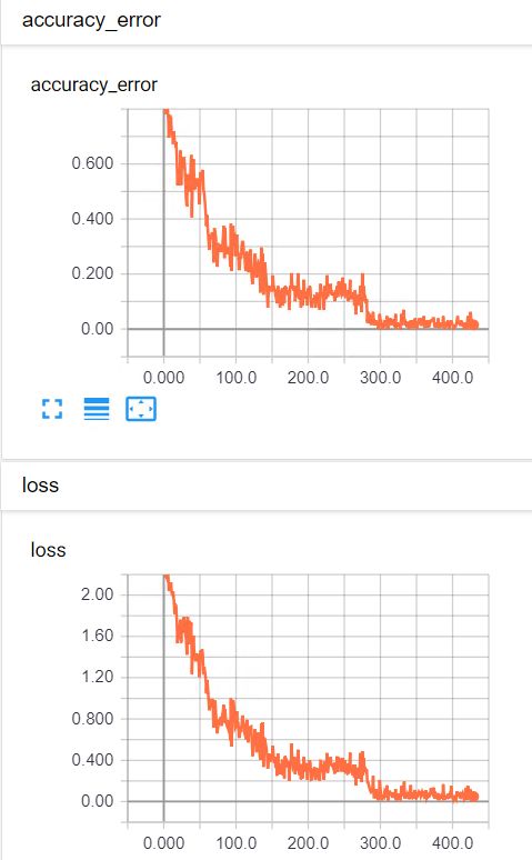
上述使用Dropout已經可以達到還不錯效果。而在2015時有人提出Batch Normalization,計算出資料的相依性並減少預設權重的影響度,在過往計算完後我們會直接計算輸出函數(softmax等等),然而每個神經元之間在輸出函數之前並沒有依賴關西,而BN就是在此層的每個神經元分布關西,而這時候預設得權重影響就會大幅降低。以下舉個例子。
假如有一向量A為[1, 3, 5]與向量B為[100, 300, 500]。
向量A:
向量B:
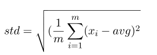
從上述例子可以看到,將資料轉為離散分布可找出資料之間的差距和與別的資料的差距,而通常都會使用標準差,其中一個原因是因為可微分,而它還有兩個參數在控制離散的線性方程式,分別為alpha和beta,可看為權重和偏權重,預設分別為1和0。
主要修改layer和conv2d的程式碼。
捲積批量正規化
moments回傳已經計算好的平均和離均差分別指派給batch_mean和batch_var。ExponentialMovingAverage為計算平滑類別[decay * pre_value - (1 - decay) * now_value],decay為損失率,這裡主要拿來記錄平均和離均的變化,平滑主要將曲線拉得比較直,可比較好觀測。此公式概念與Momentum類似。ema_apply_op為使用apply計算[]內目前的值,若[]內值沒變動則不會改變,也可以說是帶上面的公式結果還是相同。mean_var_with_update函數為返回一組與batch_mean和batch_var一樣的op,而每次使用這兩個都會觸動ema_apply_op,因為使用了control_dependencies,可以解釋為執行batch_mean或batch_var會先執行control_dependencies內參數,如此一來就能追蹤batch_mean和batch_var。而identity是搭配control_dependencies讓它生效所使用(tensorflow的機制,詳細可找相關文章閱讀)。cond是tensorflow的條件,True回傳mean_var_with_update,否回傳ema_mean, ema_var,這裡用來判斷是不是在訓練,是訓練就紀錄batch_mean和batch_var的變化。batch_norm_with_global_normalization,參數依序分別為輸入資料、均值、離均差、beta、gamma、防止除以0的被加數、是否乘上gamma。def conv_batch_norm(x, n_out, train):
beta = tf.get_variable("beta", [n_out], initializer=tf.constant_initializer(value=0.0, dtype=tf.float32))
gamma = tf.get_variable("gamma", [n_out], initializer=tf.constant_initializer(value=1.0, dtype=tf.float32))
batch_mean, batch_var = tf.nn.moments(x, [0,1,2], name='moments')
ema = tf.train.ExponentialMovingAverage(decay=0.9)
ema_apply_op = ema.apply([batch_mean, batch_var])
ema_mean, ema_var = ema.average(batch_mean), ema.average(batch_var)
def mean_var_with_update():
with tf.control_dependencies([ema_apply_op]):
return tf.identity(batch_mean), tf.identity(batch_var)
mean, var = tf.cond(train, mean_var_with_update, lambda:(ema_mean, ema_var))
normed = tf.nn.batch_norm_with_global_normalization(x, mean, var, beta, gamma, 1e-3, True)
mean_hist = tf.summary.histogram("meanHistogram", mean)
var_hist = tf.summary.histogram("varHistogram", var)
return normed
全鏈結層批量正規化
與捲積批量差別在於moments只需要取一維,還有最後使用batch_norm_with_global_normalization要轉為四維陣列。
def layer_batch_norm(x, n_out, is_train):
    beta = tf.get_variable("beta", [n_out], initializer=tf.zeros_initializer())
    gamma = tf.get_variable("gamma", [n_out], initializer=tf.ones_initializer())

    batch_mean, batch_var = tf.nn.moments(x, [0], name='moments')
    ema = tf.train.ExponentialMovingAverage(decay=0.9)
    ema_apply_op = ema.apply([batch_mean, batch_var])
    ema_mean, ema_var = ema.average(batch_mean), ema.average(batch_var)

    def mean_var_with_update():
        with tf.control_dependencies([ema_apply_op]):
            return tf.identity(batch_mean), tf.identity(batch_var)
    mean, var = tf.cond(is_train, mean_var_with_update, lambda:(ema_mean, ema_var))

    x_r = tf.reshape(x, [-1, 1, 1, n_out])
    normed = tf.nn.batch_norm_with_global_normalization(x_r, mean, var, beta, gamma, 1e-3, True)
    return tf.reshape(normed, [-1, n_out])
捲積層修改
def conv2d(input, weight_shape):
    size = weight_shape[0] * weight_shape[1] * weight_shape[2]
    weights_init = tf.random_normal_initializer(stddev=np.sqrt(2. / size))
    biases_init = tf.zeros_initializer()
    weights = tf.get_variable(name="weights", shape=weight_shape, initializer=weights_init)
    biases = tf.get_variable(name="biases", shape=weight_shape[3], initializer=biases_init)

    conv_out = tf.nn.conv2d(input, weights, strides=[1, 1, 1, 1], padding='SAME')
    conv_add = tf.nn.bias_add(conv_out, biases)
    conv_batch = conv_batch_norm(conv_add, weight_shape[3], tf.constant(True, dtype=tf.bool))
    output = tf.nn.relu(conv_batch)

    return output
全鏈結層修改
def layer(x, weights_shape):
    init = tf.random_normal_initializer(stddev=np.sqrt(2. / weights_shape[0]))
    weights = tf.get_variable(name="weights", shape=weights_shape, initializer=init)
    biases = tf.get_variable(name="biases", shape=weights_shape[1], initializer=init)
    mat_add = tf.matmul(x, weights) + biases
    mat_batch = layer_batch_norm(mat_add, weights_shape[1], tf.constant(True, dtype=tf.bool))
    output = tf.nn.relu(mat_batch)

    return output
預測函數修改
將Dropout拿掉。
def predict(x, keep_drop):
    x = tf.reshape(x, shape=[-1, 28, 28, 1])
    with tf.variable_scope("conv1_scope"):
        conv1_out = conv2d(x, conv1_size)
        pool1_out = max_pool(conv1_out)

    with tf.variable_scope("conv2_scope"):
        conv2_out = conv2d(pool1_out, conv2_size)
        pool2_out = max_pool(conv2_out)

    with tf.variable_scope("hide3_scope"):
        pool2_flat = tf.reshape(pool2_out, [-1, hide3_size[0]])
        hide3_out = layer(pool2_flat, hide3_size)
        #hide3_drop = tf.nn.dropout(hide3_out,keep_drop)

    with tf.variable_scope("out_scope"):
        output = layer(hide3_out, [hide3_size[1], output_size])

    return output
與使用Dropout相比,訓練速度提升不少,只訓練100次準確率高達98%以上,全部訓練完為99%以上,而且很穩定。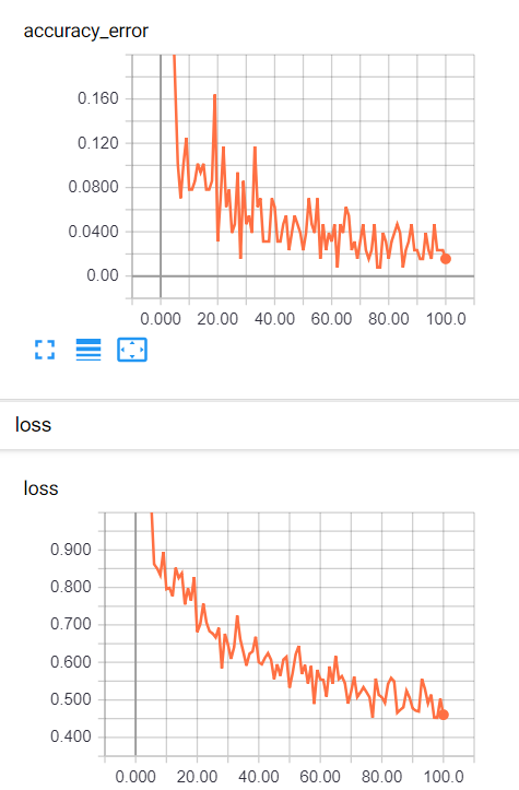
這次只使用mnist資料來測試,在書上說明可用CIFAR-10來去測試因為它有RGB三通道,而mnist只有單通道,但原理是相同的,當然也可以把自己想要訓練的資料拿來訓練,最後祝大家新年愉快,若有問題歡迎提問或私訊。
[1] https://www.tensorflow.org/api_docs/python/tf
[2] 籃子軒(譯者)(2018)。Deep Learning深度學習基礎|設計下一代人工智慧演算法。台灣:歐萊禮。
[3] https://upmath.me/
[4] https://ithelp.ithome.com.tw/articles/10199130
 Kevin
Kevin

 iThome鐵人賽