瞭解上述功能與應用後,我們會從基礎數學理論開始說起。其中包括:
所有預測模型,都離不開下圖 10 大步驟。此章節會依序解釋每個步驟的應用。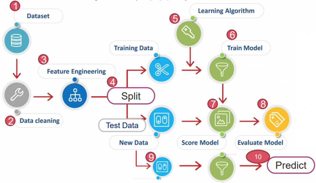
深度學習根據情境不同,概略分為三種:
資料經過 Lebaling 標籤化,即有正確解答。
此外,依據資料類型不同,監督式學習分為以下兩種:
資料集以"有限的類別"分布,對於其做歸類,即分類。如:鐵達尼號、紅酒分類...等。
以下會用兩個範例說明:
import pandas as pd
import numpy as np
from sklearn import datasets     # 引用 Scikit-Learn 中的 套件 datasets

# 1. Data Set
ds = datasets.load_iris()        # dataset: 引用 datasets 中的函數 load_iris
print(ds.DESCR)                  # DESCR: description,描述載入內容

X =pd.DataFrame(ds.data, columns=ds.feature_names)
y = ds.target

# 2. Data clean (missing value check)
print(X.isna().sum())
>>  sepal length (cm)    0
    sepal width (cm)     0
    petal length (cm)    0
    petal width (cm)     0
    dtype: int64

# 3. Feature Engineering
# No need

# 4. Data Split (Training data & Test data)
from sklearn.model_selection import train_test_split

# test_size=0.2: 測試用資料為 20%
X_train, X_test, y_train, y_test = train_test_split(X, y, test_size = 0.2)

print(X_train.shape, y_train.shape)

>>  (120, 4) (120,)

# 5. Define and train the KNN model
from sklearn.neighbors import KNeighborsClassifier

# n_neighbors=: 超參數 (hyperparameter)
clf = KNeighborsClassifier(n_neighbors = 3)

# 適配 (訓練),迴歸/分類/降維...皆用 fit()
clf.fit(X_train, y_train)

# algorithm.score: 使用 test 資料 input,並根據結果評分
print(f'score={clf.score(X_test, y_test)}')

>>  score=0.9

# 驗證答案
print(' '.join(y_test.astype(str)))
print(' '.join(clf.predict(X_test).astype(str)))

>>  1 2 0 0 0 2 1 1 1 0 1 2 2 2 0 2 1 1 1 0 1 1 2 2 1 1 0 2 2 2
    1 2 0 0 0 2 1 1 1 0 1 1 2 2 0 2 1 1 1 0 1 1 2 2 1 2 0 2 1 2

# 查看預測的機率
print(clf.predict_proba(X_test.head()))  # 預測每個 x_test 機率

>>  [[0. 1. 0.]
     [0. 0. 1.]
     [1. 0. 0.]
     [1. 0. 0.]
     [1. 0. 0.]]
import pandas as pd
import numpy as np
from sklearn import datasets

# 1. Dataset
ds = datasets.load_breast_cancer()
X =pd.DataFrame(ds.data, columns=ds.feature_names)
y = ds.target

# 2. Data clean
# no need

# 3. Feature Engineering
# no need

# 4. Split
from sklearn.model_selection import train_test_split
X_train, X_test, y_train, y_test = train_test_split(X, y, test_size = 0.2)

# 5. Define and train the KNN model
from sklearn.neighbors import KNeighborsClassifier

clf = KNeighborsClassifier(n_neighbors = 3)

# 適配(訓練),迴歸/分類/降維...皆用 fit(x_train, y_train)
clf.fit(X_train, y_train)

# algorithm.score: 使用 test 資料 input,並根據結果評分
print(f'score={clf.score(X_test, y_test)}')

>>  score=0.9210526315789473

# 驗證答案
print(' '.join(y_test.astype(str)))
print(' '.join(clf.predict(X_test).astype(str)))

>>  1 1 0 0 0 ... 0
    1 1 0 0 0 ... 0

# 查看預測的機率
print(clf.predict_proba(X_test.head()))

>>  [[0. 1.]
     [0. 1.]
     [1. 0.]
     [1. 0.]
     [1. 0.]]
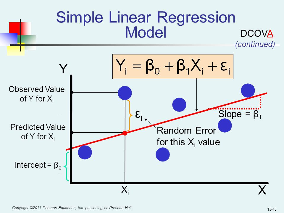
資料集以"連續的方式分布",對於其以線性方式描述,即迴歸。如:房價預測、小費預測...等。
以下會用兩個範例說明:
# 1. DataSet
year=[1950, 1951, 1952, 1953, 1954, 1955, 1956, 1957, 1958, 1959, 1960, 1961, 1962, 1963, 1964, 1965, 1966, 1967, 1968, 1969, 1970, 1971, 1972, 1973, 1974, 1975, 1976, 1977, 1978, 1979, 1980, 1981, 1982, 1983, 1984, 1985, 1986, 1987, 1988, 1989, 1990, 1991, 1992, 1993, 1994, 1995, 1996, 1997, 1998, 1999, 2000, 2001, 2002, 2003, 2004, 2005, 2006, 2007, 2008, 2009, 2010, 2011, 2012, 2013, 2014, 2015, 2016, 2017, 2018, 2019, 2020, 2021, 2022, 2023, 2024, 2025, 2026, 2027, 2028, 2029, 2030, 2031, 2032, 2033, 2034, 2035, 2036, 2037, 2038, 2039, 2040, 2041, 2042, 2043, 2044, 2045, 2046, 2047, 2048, 2049, 2050, 2051, 2052, 2053, 2054, 2055, 2056, 2057, 2058, 2059, 2060, 2061, 2062, 2063, 2064, 2065, 2066, 2067, 2068, 2069, 2070, 2071, 2072, 2073, 2074, 2075, 2076, 2077, 2078, 2079, 2080, 2081, 2082, 2083, 2084, 2085, 2086, 2087, 2088, 2089, 2090, 2091, 2092, 2093, 2094, 2095, 2096, 2097, 2098, 2099, 2100]
pop=[2.53, 2.57, 2.62, 2.67, 2.71, 2.76, 2.81, 2.86, 2.92, 2.97, 3.03, 3.08, 3.14, 3.2, 3.26, 3.33, 3.4, 3.47, 3.54, 3.62, 3.69, 3.77, 3.84, 3.92, 4.0, 4.07, 4.15, 4.22, 4.3, 4.37, 4.45, 4.53, 4.61, 4.69, 4.78, 4.86, 4.95, 5.05, 5.14, 5.23, 5.32, 5.41, 5.49, 5.58, 5.66, 5.74, 5.82, 5.9, 5.98, 6.05, 6.13, 6.2, 6.28, 6.36, 6.44, 6.51, 6.59, 6.67, 6.75, 6.83, 6.92, 7.0, 7.08, 7.16, 7.24, 7.32, 7.4, 7.48, 7.56, 7.64, 7.72, 7.79, 7.87, 7.94, 8.01, 8.08, 8.15, 8.22, 8.29, 8.36, 8.42, 8.49, 8.56, 8.62, 8.68, 8.74, 8.8, 8.86, 8.92, 8.98, 9.04, 9.09, 9.15, 9.2, 9.26, 9.31, 9.36, 9.41, 9.46, 9.5, 9.55, 9.6, 9.64, 9.68, 9.73, 9.77, 9.81, 9.85, 9.88, 9.92, 9.96, 9.99, 10.03, 10.06, 10.09, 10.13, 10.16, 10.19, 10.22, 10.25, 10.28, 10.31, 10.33, 10.36, 10.38, 10.41, 10.43, 10.46, 10.48, 10.5, 10.52, 10.55, 10.57, 10.59, 10.61, 10.63, 10.65, 10.66, 10.68, 10.7, 10.72, 10.73, 10.75, 10.77, 10.78, 10.79, 10.81, 10.82, 10.83, 10.84, 10.85]
df = pd.DataFrame({'year' : year, 'pop' : pop})
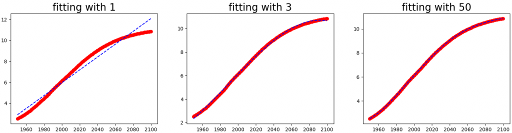
# 2. 求 1 次項均方誤差 MSE (Mean-Square Error)
in_year = int(input('Please input 1950~2100 to calculation:'))
fit1 = np.polyfit(x, y, 1)
if 2100 >= in_year >= 1950:
print('The actual pop is:', y[in_year-1950])
print('Predict pop is:', f'{(np.poly1d(fit1)(in_year)):.2}')
y1 = fit1[0]*np.array(x) + fit1[1]
print('MSE is:', f'{((y - y1)**2).mean():.2}')
else:
print('Wrong year!')
# 3. 作圖
def ppf(x, y, order):
fit = np.polyfit(x, y, order) # 線性迴歸,求 y=a + bx^1+ cx^2 ...的參數
p = np.poly1d(fit) # 將 polyfit 迴歸解代入
t = np.linspace(1950, 2100, 2000)
plt.plot(x, y, 'ro', t, p(t), 'b--')
plt.figure(figsize=(18, 4))
titles = ['fitting with 1', 'fitting with 3', 'fitting with 50']
for i, o in enumerate([1, 3, 50]):
plt.subplot(1, 3, i+1)
ppf(year, pop, o)
plt.title(titles[i], fontsize=20)
plt.show()
import pandas as pd
import numpy as np
from sklearn import datasets

# 1. Dataset
ds = datasets.load_boston()
X =pd.DataFrame(ds.data, columns=ds.feature_names)
y = ds.target

# 2. Data clean
print(X.isna().sum())

# 3. Feature Engineering

# 4. Split
from sklearn.model_selection import train_test_split
X_train, X_test, y_train, y_test = train_test_split(X, y, test_size = 0.2)
>> (404, 13) (404,)

# 5. Define and train the LinearRegression model
from sklearn.linear_model import LinearRegression

clf = LinearRegression()

# 適配(訓練),迴歸/分類/降維...皆用 fit(x_train, y_train)
clf.fit(X_train, y_train)

# algorithm.score: 使用 test 資料 input,並根據結果評分
print(f'score={clf.score(X_test, y_test)}')
>> import pandas as pd
import numpy as np
from sklearn import datasets

# 1. Dataset
ds = datasets.load_boston()
X =pd.DataFrame(ds.data, columns=ds.feature_names)
y = ds.target

# 2. Data clean
print(X.isna().sum())

# 3. Feature Engineering

# 4. Split
from sklearn.model_selection import train_test_split
X_train, X_test, y_train, y_test = train_test_split(X, y, test_size = 0.2)
>> (404, 13) (404,)

# 5. Define and train the LinearRegression model
from sklearn.linear_model import LinearRegression

clf = LinearRegression()

# 適配(訓練),迴歸/分類/降維...皆用 fit(x_train, y_train)
clf.fit(X_train, y_train)

# algorithm.score: 使用 test 資料 input,並根據結果評分
print(f'score={clf.score(X_test, y_test)}')

>>  score=0.6008214413101689

# 驗證答案
print(list(y_test))
b = [float(f'{i:.2}') for i in clf.predict(X_test)]
print(b)

>>  [30.3, 8.4, 17.4, 10.2, 12.8, ... 22.5]
    [32.0, 4.6, 22.0, 6.2, 13.0, ... 29.0]
部分或者全部資料 Unlebaling 無標籤化,即沒有正確解答。
將特徵相近的點歸類,概念有些類似 Regression,稱為集群。如下圖: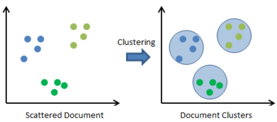
以下為 CLV (Regression) 範例:
import numpy as np
import pandas as pd
import matplotlib.pyplot as plt
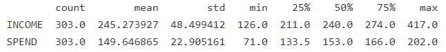
ds = pd.read_csv('CLV.csv')
print(ds.describe().T)
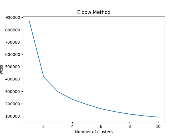
分 1~10群,計算誤差平方和 (elbow method) 最少者為優。
# 沒有 y
X=ds.iloc[:,[0,1]].values


from sklearn.cluster import KMeans
wcss = []
for i in range(1,11):
    km=KMeans(n_clusters=i, init='k-means++', max_iter=300, n_init=10, random_state=0)
    km.fit(X)
    wcss.append(km.inertia_)
plt.plot(range(1,11),wcss)
plt.title('Elbow Method')
plt.xlabel('Number of clusters')
plt.ylabel('wcss')
plt.show()
使用 sklearn 內建計算輪廓係數 (Silhoutte Coefficient)
from sklearn.metrics import silhouette_score
from sklearn.cluster import KMeans

for n_cluster in range(2, 11):
    kmeans = KMeans(n_clusters=n_cluster).fit(X)
    label = kmeans.labels_
    sil_coeff = silhouette_score(X, label, metric='euclidean')
    print(f"n_clusters={n_cluster}, Silhouette Coefficient is {sil_coeff:.4}")

>>  n_clusters=2, Silhouette Coefficient is 0.4401
    n_clusters=3, Silhouette Coefficient is 0.3596
    n_clusters=4, Silhouette Coefficient is 0.3721
    n_clusters=5, Silhouette Coefficient is 0.3617
    n_clusters=6, Silhouette Coefficient is 0.3632
    n_clusters=7, Silhouette Coefficient is 0.3629
    n_clusters=8, Silhouette Coefficient is 0.3538
    n_clusters=9, Silhouette Coefficient is 0.3441
    n_clusters=10, Silhouette Coefficient is 0.3477
若要視覺化分群,可見以下
# Fitting kmeans to the dataset
km4=KMeans(n_clusters=8,init='k-means++', max_iter=300, n_init=10, random_state=0)
y_means = km4.fit_predict(X)

# Visualising the clusters for k=4
plt.scatter(X[y_means==0,0],X[y_means==0,1],s=50, c='purple',label='Cluster1')
plt.scatter(X[y_means==1,0],X[y_means==1,1],s=50, c='blue',label='Cluster2')
plt.scatter(X[y_means==2,0],X[y_means==2,1],s=50, c='green',label='Cluster3')
plt.scatter(X[y_means==3,0],X[y_means==3,1],s=50, c='cyan',label='Cluster4')
plt.scatter(X[y_means==4,0],X[y_means==4,1],s=50, c='yellow',label='Cluster5')
plt.scatter(X[y_means==5,0],X[y_means==5,1],s=50, c='black',label='Cluster6')
plt.scatter(X[y_means==6,0],X[y_means==6,1],s=50, c='brown',label='Cluster7')
plt.scatter(X[y_means==7,0],X[y_means==7,1],s=50, c='red',label='Cluster8')

plt.scatter(km4.cluster_centers_[:,0], km4.cluster_centers_[:,1],s=200,marker='s', c='red', alpha=0.7, label='Centroids')
plt.title('Customer segments')
plt.xlabel('Annual income of customer')
plt.ylabel('Annual spend from customer on site')
plt.legend()
plt.show()
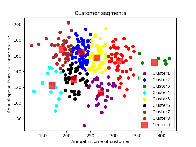
Note: 一般客戶分析會使用 RFM (Recency-Frequency-Monetary) 分析
此為機器學習第三步:Feature Engineering
讓機器學習算法,自動學會對環境做出反應。
由於是初學,因此會先聚焦在**"監督式學習"&"非監督式學習"**上。
以上就是程式基礎簡介,下篇將從理論基礎開始介紹。
.
.
.
.
.
請使用 sklearn 內建的 Datasets,依照上述步驟完成以下資料的迴歸or分類:
提示:ds = datasets.load_wine()
提示:ds = datasets.load_diabetes()
提示:ds = datasets.load_tips()
.
.
.
.
.
 s790502ss

 iThome鐵人賽