import numpy as np
from matplotlib import pyplot as plt
def rate(x):
    return x**2 + x

t1 = np.array(range(0, 11))
t2 = np.array([2,7])
r = (rate(11)-rate(0))/(11 - 0)   # 求平均斜率 (t1)

# 作圖
plt.xlabel('Seconds')
plt.ylabel('Meters')
plt.grid()
plt.plot(t1, rate(t1), c='g')
plt.plot(t2, rate(t2), c='m')
plt.annotate(f'Average Velocity = {str(r)} m/s',((11+0)/2, (rate(11)+rate(0))/2))
plt.show()
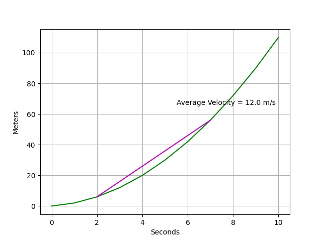
此結果因取樣間隔過大,導致算出來的速度變化率失準。
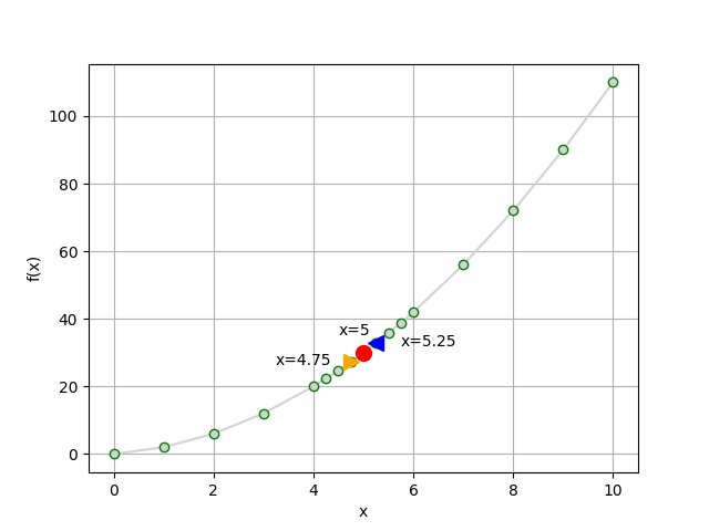
同上例,這次取樣更密集
import matplotlib.pyplot  as plt
def f(x):
    return x**2 + x

# 加點點
add = [4.25, 4.5, 4.75, 5,  5.25, 5.5, 5.75]
x = list(range(0,5)) + add + list(range(6,11))
y = [f(i) for i in x]

# 作圖
plt.xlabel('x')
plt.ylabel('f(x)')
plt.grid()
plt.plot(x, y, c='lightgrey', marker='o', markeredgecolor='g') # , markerfacecolor='green'

# Plot f(x) when x = 5
plt.plot(5, f(5), c='r', marker='o', markersize=10)
plt.annotate('x=' + str(5),(5, f(5)), xytext=(5-0.5, f(5)+5))
# Plot f(x) when x = 5.25
plt.plot(5.25, f(5.25), c='b', marker='<', markersize=10)
plt.annotate('x=' + str(5.25),(5.25, f(5.25)), xytext=(5.25+0.5, f(5.25)-1))
# Plot f(x) when x = 4.75
plt.plot(4.75, f(4.75), c='orange', marker='>', markersize=10)
plt.annotate('x=' + str(4.75),(4.75, f(4.75)), xytext=(4.75-1.5, f(4.75)-1))

plt.show()
def g(x):
    if x != 0:
        return -(12/(2*x))**2

import matplotlib.pyplot as plt

x = range(-20, 21)
y = [g(a) for a in x]

# 作圖
plt.xlabel('x')
plt.ylabel('g(x)')
plt.grid()
plt.plot(x, y, c='m')

plt.show()
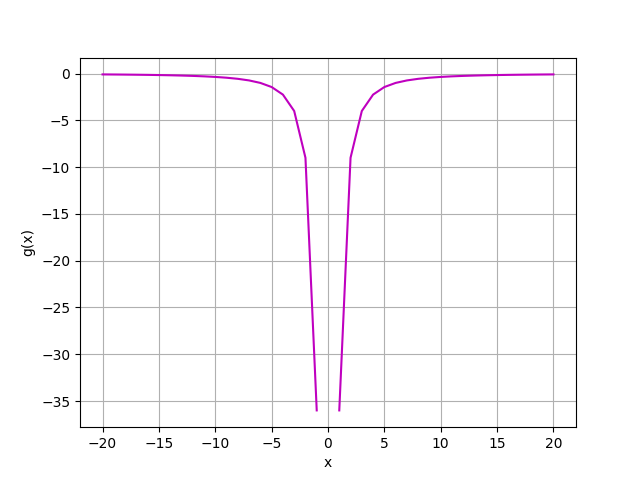
此函數於 x=0 不存在極限值,故為一"不連續函數"
A. Basic
import sympy as sp
import numpy as np

def lim(x_value):
    x = sp.Symbol('x')
    y = (x**3 - 2*x**2 + x) / x**2 -1
    return sp.limit(y, x, x_value)
print(lim(2))

>>  -1/2
B. 無窮
import sympy as sp
import numpy as np

def lim(x_value):
    x = sp.Symbol('x')
    y = ((x**4)-3*(x**3)-x+3) / ((x**3)-9*x)
    return sp.limit(y, x, x_value)
print(lim(0))

>>  -oo   # 負無限大
C. 善用 if 規避無極限值
import sympy as sp
import numpy as np

def lim(x_value):
    if x_value != 1:
        x = sp.Symbol('x')
        y = (3*x**3 - 3) / (3**x - 3)
        return sp.limit(y, x, x_value)
    else:
        return 'fuck'
print(lim(1))

>>  fuck
import matplotlib.pyplot as plt
def f(x):
return x**2 + x
x = list(range(0, 11))
y = [f(i) for i in x]
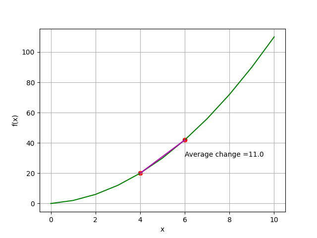
# 指定任意兩點 f(4) & f(6)
x1, x2 = 4, 6
y1, y2 = f(x1), f(x2)
slope = (y2 - y1)/(x2 - x1)
sx = [x1, x2]
sy = [f(i) for i in sx]
# 作圖
plt.xlabel('x')
plt.ylabel('f(x)')
plt.grid()
plt.plot(x, y, 'g', sx, sy, 'm') # 畫出 f(x) & f(6)-f(4)
plt.scatter([x1, x2], [y1, y2], c='r')
plt.annotate('Average change =' + str(slope),(x2, (y2+y1)/2))
plt.show()
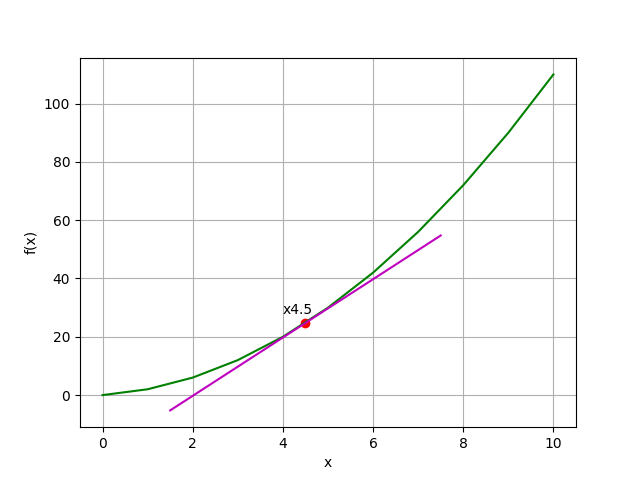
import matplotlib.pyplot as plt

def f(x):
    return x**2 + x

x = list(range(0, 11))
y = [f(i) for i in x]

x1, x2 = 4.5, 4.5000000001
y1, y2 = f(x1), f(x2)

# 作圖
plt.xlabel('x')
plt.ylabel('f(x)')
plt.grid()
plt.plot(x, y, c='g')
plt.scatter(x1, y1, c='r')

# 為方便表示,放大切線長度
m = (y2-y1)/(x2-x1)
xMin, xMax = x1 - 3, x1 + 3
yMin, yMax = y1 - (3*m), y1 + (3*m)
plt.plot([xMin, xMax],[yMin, yMax], c='m')
plt.annotate('x' + str(x1),(x1, y1), xytext=(x1-0.5, y1+3))

plt.show()
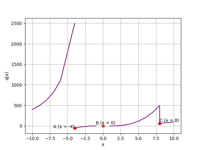
要滿足可微性,函數必須包含:
import matplotlib.pyplot as plt

def q(x):
    if x != 0:
        if x < -4:
            return 40000 / (x**2)
        elif x < 8:
            return (x**2 - 2) * x - 1
        else:
            return (x**2 - 2)

x1 = list(range(-10, -5)) + [-4.0001]
x2 = list(range(-4,8)) + [7.9999] + list(range(8,11))
y1 = [q(i) for i in x1]
y2 = [q(i) for i in x2]

# 作圖
plt.xlabel('x')
plt.ylabel('q(x)')
plt.grid()

# 紫線
plt.plot(x1, y1, c='purple')
plt.plot(x2, y2, c='purple')

# 紅點
xp = [-4, 0, 8]
yp = [q(-4), 0, q(8)]
plt.scatter(xp, yp, c='r')
plt.annotate('A (x = -4)',(-5, q(-3.9)), xytext=(-7, q(-3.9)))   # 切線為垂直
plt.annotate('B (x = 0)',(0, 0), xytext=(-1, 40))                # 不連續
plt.annotate('C (x = 8)',(8, q(8)), xytext=(8, 100))             # 不平滑

plt.show()
f(x) = 6
∴ f'(x) = 0
f(x) = 2g(x)
∴ f′(x) = 2g′(x)
f(x) = [g(x) + h(x)]
∴ f'(x) = g'(x) + h'(x)
f(x) = x^n
∴ f′(x) = nx^(n-1)
** [f(x)g(x)]' = f′(x)g(x) + f(x)g'(x)**
證明如下:
令 t→x
[f(x)g(x)]'
    = [f(t)g(t) - f(x)g(x)] / (t-x)
    = {f(t)g(t) + [f(x)g(t) - f(x)g(t)] - f(x)g(x)} / (t-x)
    = {g(t)[f(t) - f(x)] + f(x)[g(t) - g(x)} / (t-x)

又 t→x,上述算式變為
    → f′(x)g(x) + f(x)g'(x)
** [f(x)/g(x)]' = [f'(x)g(x) - g'(x)f(x)] / g(x)^2**
證明如下:
令 t→x
[f(x)/g(x)]'
    = [f(t)/g(t) - f(x)g(x)] / (t-x)
    = [f(t)g(x) - f(x)g(t)] / g(t)g(x)(t-x)
    = {f(t)g(x) + [f(t)g(t) - f(t)g(t)] - f(x)g(t)} / g(t)g(x)(t-x)
    = {-f(t)[g(t) - g(x)] + g(t)[f(t) - f(x)]}  / g(t)g(x)(t-x)

又 t→x,上述算式變為
    → [f'(x)g(x) - g'(x)f(x)] / g(x)^2
f(u) = u(g(x))
[f(x)]' = f'(u)g'(x)
證明如下:
令 t→x, 且 g(t)=v, g(x)=u
[f(x)]'
    = [f(v) - f(u)] / (t - x)
    # 擴分 [g(t) - g(x)]/[g(t) - g(x)]
    = [f(v) - f(u)] / [g(t) - g(x)] * [g(t) - g(x)] / (t - x)
    = [f(v) - f(u)] / (v - u) * [g(t) - g(x)] / (t - x)

又 t→x,所以 v→u,,上述算式變為
→ f'(u) * g'(x)
import sympy as sp
import numpy as np

# 1. 微分方程式結果 f'(x)
x = sp.Symbol('x')
y = 3*x**2 + 2
yprime = y.diff(x)
print(yprime)
>> 6*x

# 2. 用 sub() 代入 x
x = sp.Symbol('x')
y = 3*x**3 + 2 * x
yprime = y.diff(x)
print(yprime.subs({x:7}))
>> 443

# 3. 用 lambdify() 代入多個 x
f = sp.lambdify(x, yprime, 'numpy')
l = [1, 3, 5, 7, 10]
print(f(np.array(l)))      # 代入 x 計算 f'(x)
>> [ 11  83 227 443 902]
.
.
.
.
.
(https://reurl.cc/DgbDqe)
Ex.1-1 (2i):(x+2)(x-3) = (x-5)(x-6)
Ex.1-2 (3c):|10-2x| = 6
(https://reurl.cc/EnbDQk)
Ex.2-1 (3c):
4x + 3y = 4
2x + 2y - 2z = 0
5x + 3y + z = -2
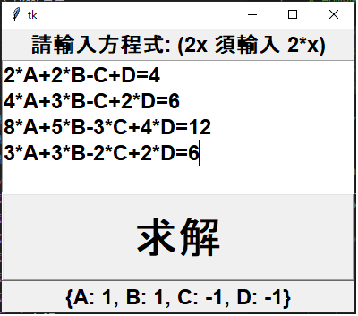
Ex.2-2 (4a):
2a + 2b - c + d = 4
4a + 3b - c + 2d = 6
8a + 5b - 3c + 4d = 12
3a + 3b -2c + 2d = 6
 s790502ss

 iThome鐵人賽