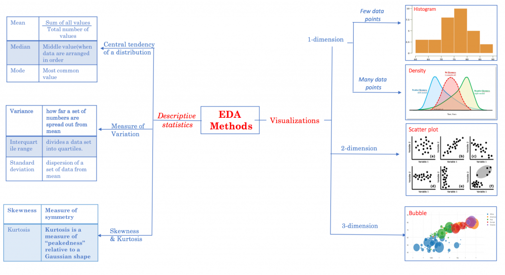
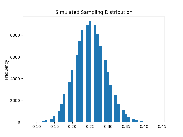
不論任何分配的母體,若樣本夠大,則每批樣本的平均值 (X_bar) 的機率分配都會趨近常態分配(normal distribution)。
EX1. 抽取 10,000 批,每批 100 個樣本,成功機率 0.25。
# 二項分配隨機抽樣 np.random.binomial(n, p, s)
# n: 每次抽樣樣本數
# p: 樣本分配(母體機率)
# s: 抽樣次數

import pandas as pd
import matplotlib.pyplot as plt
import numpy as np

n, p, s = 100, 0.25, 100000
X = np.random.binomial(n, p, s)   # return 每次抽樣成功次數 X
X_mean = X/n  # 樣本平均值

df = pd.DataFrame(X_mean, columns=['p-hat'])
print(df)

means = df['p-hat']
means.plot(kind='hist', title='Simulated Sampling Distribution', bins=50)
plt.savefig('pic 4-5 1')
plt.show()

print (f'Mean: {means.mean():.3f}')
>>  Mean: 0.250
print (f'Std: {means.std():.3f}')
>>  Std: 0.043
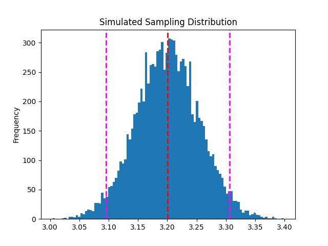
基於某一信心水準(confidence level),例如95%,我們確信真實的參數值會落在特定區間內,稱之。
信賴區間 = standard error x Z score
import pandas as pd
import matplotlib.pyplot as plt
import numpy as np
from scipy import stats

mu, sigma, n = 3.2, 1.2, 500
samples = list(range(0, 10000)) # 抽幾次

X = np.array([])
X_bar = np.array([])

# np.random.normal(mean, std, n),return n-d array
for s in samples:
    sample = np.random.normal(mu, sigma, n)
    X = np.append(X, sample)
    X_bar = np.append(X_bar, sample.mean())

df = pd.DataFrame(X_bar, columns=['X_bar'])

# 取得 X_mean 的 mean, std, 95% 信賴區間
m = df['X_bar'].mean()                  # X_bar 的平均
se = df['X_bar'].std()                  # 標準誤
ci = stats.norm.interval(0.95, m, se)   # return [m - 1.96 std, m + 1.96 std]

print (f'Sampling Mean: {m:.3f}')
>>  Sampling Mean: 3.201
print (f'Sampling StdErr: {se:.3f}')
>>  Sampling StdErr: 0.054
print (f'95% Confidence Interval: {ci}')
>>  95% Confidence Interval: (3.095256779885818, 3.3061798693546534)

# 作圖
df['X_bar'].plot.hist(title='Simulated Sampling Distribution', bins=100)
plt.axvline(m, color='red', linestyle='dashed', linewidth=2)
plt.axvline(ci[0], color='magenta', linestyle='dashed', linewidth=2)
plt.axvline(ci[1], color='magenta', linestyle='dashed', linewidth=2)
plt.show()
首先有幾個名詞需要了解:
確認偏誤(Confirmation Bias):人根據主觀感受,而非客觀資訊建立起主觀以為的社會現實。
邏輯公理:
矛盾率:命題不可又真又假
排中率:命題只可以真或假
根據矛盾率,可以由假命題反證明真命題。
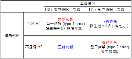
Null Hypothesis 虛無假設(H0):主張「母群參數與某數字之間無差別」
Alternative Hypothesis 對立假設(H1):主張「母群參數與某數字之間有差別」
虛無假設與對立假設兩者必須互斥(有 A 沒 B)且窮盡(包含所有)
有了以上,接著我們進入假設檢定
顧名思義,單尾檢定即假設拒絕區(critical value)僅有一邊,其拒絕機率為 P。
反之,雙尾檢定即拒絕區包含兩邊,拒絕機率為 P/2。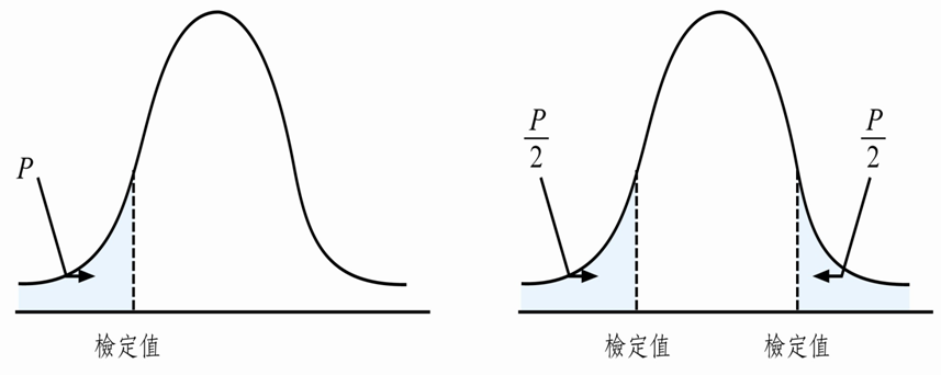
EX1. 一般人平均智商為100,標準差為15,呈常態分配。三峽典獄長挑選30位受刑人的隨機樣本,發現智商平均為95.1,請檢測: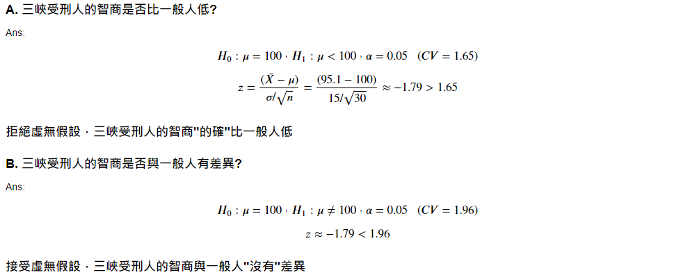
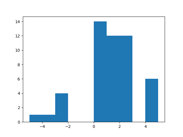
EX2. 學生為此課程打分,評分-5~5。請檢測學生是否喜歡這門課程?
A. H0: u <= 0(學生不喜歡)
B. H1: u > 0 (學生喜歡)
C. alpha = 1.645 (90%)
import numpy as np
import matplotlib.pyplot as plt

np.random.seed(123)
low = np.random.randint(-5, -1, 6)
mid = np.random.randint(0, 3, 38)
high = np.random.randint(4, 6, 6)
sample = np.append(low, np.append(mid, high))
print("Min:" + str(sample.min()))
print("Max:" + str(sample.max()))
print("Mean:" + str(sample.mean()))

plt.hist(sample)
plt.show()
from scipy import stats
import numpy as np
import matplotlib.pyplot as plt

# 樣本(平均 0、標準差 1.15、抽取 10000 次)
sample = np.random.normal(0.5, 1.15, 100)

# scipy.stats.ttest_1samp(a, mother, alternative='two-sided') # 單樣本檢定
# a: 樣本
# mother: 母體
# alternative: 'two-sided'(雙尾), 'less', 'greater'(左/右尾)
z, p = stats.ttest_1samp(sample, 0, alternative='greater')
print(f'z-statistic:{z}')
>>  z-statistic:3.9074479639245183
print(f'p-value:{p}')
>>  p-value:8.53595856851376e-05

x_bar = np.random.normal(sample.mean(), sample.std(), 10000)
plt.hist(x_bar, bins=100)
plt.axvline(x_bar.mean(), c='y', linestyle='--', linewidth=2)

# 計算信心水準 95%,右尾檢定結果(右邊 5%)的 x_bar 值
ci = stats.norm.interval(0.90, 0, 1.15)   # 此函數僅能計算雙尾
plt.axvline(ci[1], c='r', linestyle='--', linewidth=2)

# 根據 mean + t*s 劃出對立假設 x_bar 落點
plt.axvline(x_bar.mean() + z*x_bar.std(), c='m', linestyle='--', linewidth=2)
plt.show()
結論:紫色落於紅色外,拒絕虛無假設。sample 有顯著大於 0。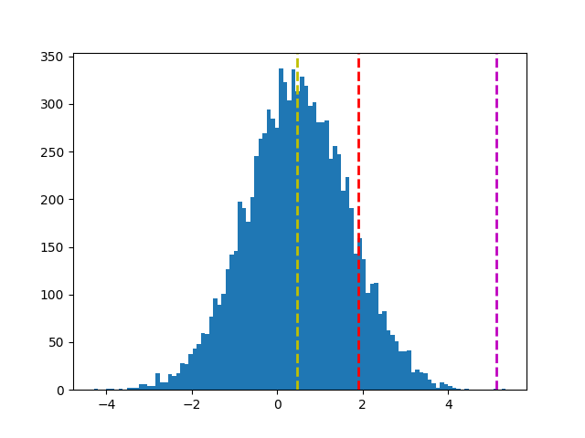
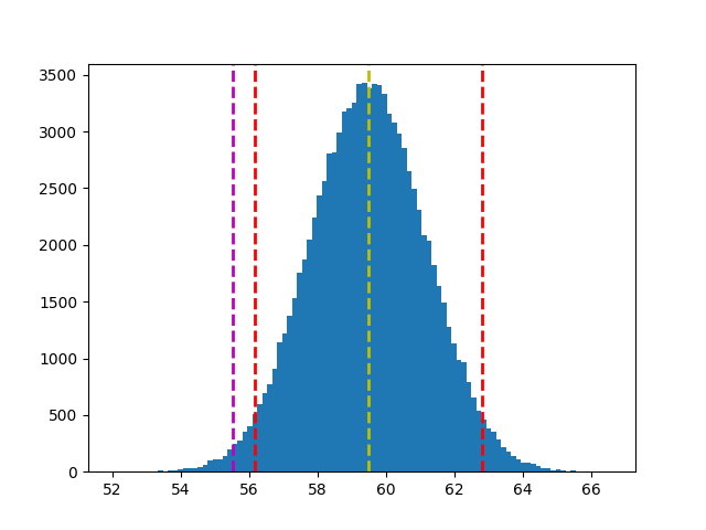
import numpy as np
import matplotlib.pyplot as plt
from scipy import stats

np.random.seed(123)
sample1 = np.random.normal(59.45, 1.5, 100)
sample2 = np.random.normal(60.05, 1.5, 100)

# scipy.stats.ttest_rel(a, b, alternative='two-sided') # 雙樣本檢定
# a & b: 樣本
# alternative: 'two-sided'(雙尾), 'less', 'greater'(左/右尾)
t, p = stats.ttest_rel(sample1, sample2)    # , alternative='greater'
print(f't-statistic:{t}')
>>  t-statistic:-2.3406857739212583
print(f'p-value:{p}')
>>  p-value:0.021254108930688475

# 根據 sample1 平均值 & 樣本標準差,劃出抽取 100000 次(每次100批)分配
s1_bar = np.random.normal(sample1.mean(), sample1.std(), 100000)
plt.hist(s1_bar, bins=100)
plt.axvline(s1_bar.mean(), c='y', linestyle='--', linewidth=2)

# 計算信心水準 95%,右尾檢定結果(一邊 5%)的 x_bar 值
ci = stats.norm.interval(0.95, s1_bar.mean(), s1_bar.std())
plt.axvline(ci[0], c='r', linestyle='--', linewidth=2)
plt.axvline(ci[1], c='r', linestyle='--', linewidth=2)

# 根據 mean + t*s 劃出對立假設 x_bar 落點
plt.axvline(s1_bar.mean() + t*s1_bar.std(), c='m', linestyle='--', linewidth=2)
plt.show()
.
.
.
.
.
#1. 今彩 539 (https://www.taiwanlottery.com.tw/dailycash/index.asp)
各獎項的中獎方式如下表: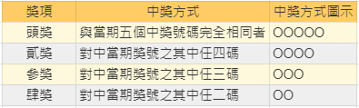
獎金如下: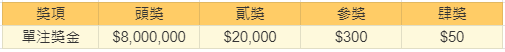
解答如下:
import scipy.special as sps
import numpy as np

name = ['頭獎', '二獎', '三獎', '四獎']
bonus = [8000000, 20000, 300, 50]
total = []
for i in range(4):
    prob = sps.comb(5, 5-i) * sps.comb(34, i) / sps.comb(39, 5)
    money = sps.comb(5, 5-i) * sps.comb(34, i) * bonus[i]
    total.append(money)
    print(f'{name[i]} 中獎機率為: {prob*100 :.4f} %')

gain = np.array(total).sum()/sps.comb(39, 5)
cost = 50

print()
print(f'平均每注中獎金額: {gain :.2f}')
print(f'平均每注投報率為: {(gain-cost)*100/cost :.2f} %')

>>  頭獎 中獎機率為: 0.0002 %
    二獎 中獎機率為: 0.0295 %
    三獎 中獎機率為: 0.9744 %
    四獎 中獎機率為: 10.3933 %

    平均每注中獎金額: 27.92
    平均每注投報率為: -44.16 %
#2. 使用 sklearn 內建資料集 "load_boston" 來預測波士頓房價
A. 一次迴歸求解:
# A-1. Data prepare 準備資料
from sklearn import datasets
ds = datasets.load_boston()

import pandas as pd
X = pd.DataFrame(ds.data, columns=ds.feature_names)
y = ds.target   # 房價

# A-2. Data clean 資料清理
print(X.isnull().sum().sum())
>>  0

# A-4. Split 拆分資料
from sklearn.model_selection import train_test_split
X_train, X_test, y_train, y_test = train_test_split(X, y, test_size = 0.2)

# A-3. Feature Engineering 特徵工程
# 標準化、歸一化,嚴謹的作法是放在 4. Split 後,以此避免訓練資料與測試資料互相干擾。
from sklearn.preprocessing import StandardScaler
scaler = StandardScaler()
X_train = scaler.fit_transform(X_train) # 訓練資料要特徵縮放
X_test = scaler.transform(X_test)       # 測試資料則僅做特徵轉換

# A-5. Train Model 機器訓練
from sklearn.linear_model import LinearRegression
clf = LinearRegression()
clf.fit(X_train, y_train)

print(clf.coef_)            # 迴歸線係數
>>  [-0.73333119  1.29309093  0.15261025  0.61015457 -2.18126673  2.48140152
      0.18613576 -3.10258233  2.78838943 -2.32101423 -1.97367244  0.76910136
     -4.00329437]
print(clf.intercept_)       # 迴歸線偏差值(截距)
>>  22.450247524752527

# 最大影響因子
import numpy as np
print(ds.feature_names[np.argmax(clf.coef_)]) # 係數最大項
>>  RAD
print(np.max(clf.coef_)[::-1])                # 值
>>  2.78838943

# A-6. Score Model
score = clf.score(X_test, y_test)
print('Model Score:', score)
>>  Model Score: 0.7445778921293265

# 計算 MSE (mean square error)
from sklearn.metrics import mean_squared_error
MSE = mean_squared_error(y_test, clf.predict(X_test))
print('MSE=', MSE)
>>  MSE= 21.285739578017278

# 均方根誤差
RMSD = mean_squared_error(y_test, clf.predict(X_test)) ** .5
print('RMSD=', RMSD)
>>  RMSD= 4.61364710159081

# 判定係數(之後會講)
from sklearn.metrics import r2_score
judge = r2_score(y_test, clf.predict(X_test))
print('R2 Score=', judge)
>>  R2 Score= 0.7445778921293265
B. 二次迴歸
一次迴歸結果看來準確率還不夠高,
我們可以用 sklearn 中的 PolynomialFeatures 調整自由度為 2:
# B-1. Data prepare 準備資料
from sklearn import datasets
ds = datasets.load_boston()

import pandas as pd
X = pd.DataFrame(ds.data, columns=ds.feature_names)
y = ds.target   # 房價

# 使用 sklearn 中的 PolynomialFeatures 轉換為二次迴歸
# 預設 degree=2,即 Y 會由 [1, a, b, a^2, ab, b^2] 組成
from sklearn.preprocessing import PolynomialFeatures
poly = PolynomialFeatures(degree=2)
X2 = poly.fit_transform(X)

# B-2. Data clean 資料清理

# B-4. Split 拆分資料
from sklearn.model_selection import train_test_split
X_train, X_test, y_train, y_test = train_test_split(X2, y, test_size = 0.2)

# B-3. Feature Engineering 特徵工程
from sklearn.preprocessing import StandardScaler
scaler = StandardScaler()
X_train = scaler.fit_transform(X_train) # 訓練資料特徵縮放
X_test = scaler.transform(X_test)       # 測試資料僅做轉換

# B-5. Train Model 機器訓練
from sklearn.linear_model import LinearRegression
clf = LinearRegression()
clf.fit(X_train, y_train)

# B-6. Score Model
score = clf.score(X_test, y_test)
print('Model Score:', score)
>>  Model Score: 0.8832125484403865

# 計算 MSE (mean square error)
from sklearn.metrics import mean_squared_error
MSE = mean_squared_error(y_test, clf.predict(X_test))
print('MSE=', MSE)
>>  MSE= 10.88594930129324

# 均方根誤差
RMSD = mean_squared_error(y_test, clf.predict(X_test)) ** .5
print('RMSD=', RMSD)
>>  RMSD= 3.299386200688431
C. 矩陣公式
最後,我們用矩陣公式 A = (X'*X)^-1*X'*Y求解:
# C-1. Data prepare 準備資料
from sklearn import datasets
ds= datasets.load_boston()

import pandas as pd
X = pd.DataFrame(ds.data, columns=ds.feature_names)
y = ds.target
# print(X.head())

# C-4. Split 拆分資料
from sklearn.model_selection import train_test_split
X_train, X_test, y_train, y_test = train_test_split(X, y, test_size = 0.2)

# C-5. 矩陣運算
# 最後一行補1
import numpy as np
b_train = np.ones((X_train.shape[0], 1))
# print(b_train.shape)          # (404, 1)
# 黏合
X_train=np.hstack((X_train, b_train))


# # 套用公式 A = (X' * X)^-1 * X' * Y
# print(X_train.T.shape)  # (14, 404)
# print(X_train.shape)    # (404, 14)
# print(y_train.T.shape)  # (404,)
A = np.linalg.inv(X_train.T @ X_train) @ X_train.T @ y_train
print(A.shape)

# matrix(X_train, y_train)


# # 計算 MSE (mean square error)
# print(X_test.shape)     # (102, 13)
# print(y_test.shape)     # (102,)

b_test = np.ones((X_test.shape[0], 1))
# print(b_test.shape)          # (102, 1)
# 黏合
X_test=np.hstack((X_test, b_test))

MSE = np.sum((X_test @ A - y_test) ** 2) / y_test.shape[0]
print('MSE=', MSE)
>>  MSE= 17.679787655718744

# 均方根誤差
RMSD = MSE ** 0.5
print('RMSD=', RMSD)
>>  RMSD= 4.204733957781246
.
.
.
.
.
使用假設檢定,檢定近40年(10屆)美國總統的身高是否有差異?
(Data: president_height.csv)
 s790502ss

 iThome鐵人賽