https://github.com/PacktPublishing/Machine-Learning-Algorithms

實作與最佳化

首先導入套件，上面的是用來算數學的;下面的是用來畫畫的，並且幫它們取綽號(np & plt)。

import numpy as np
import matplotlib.pyplot as plt

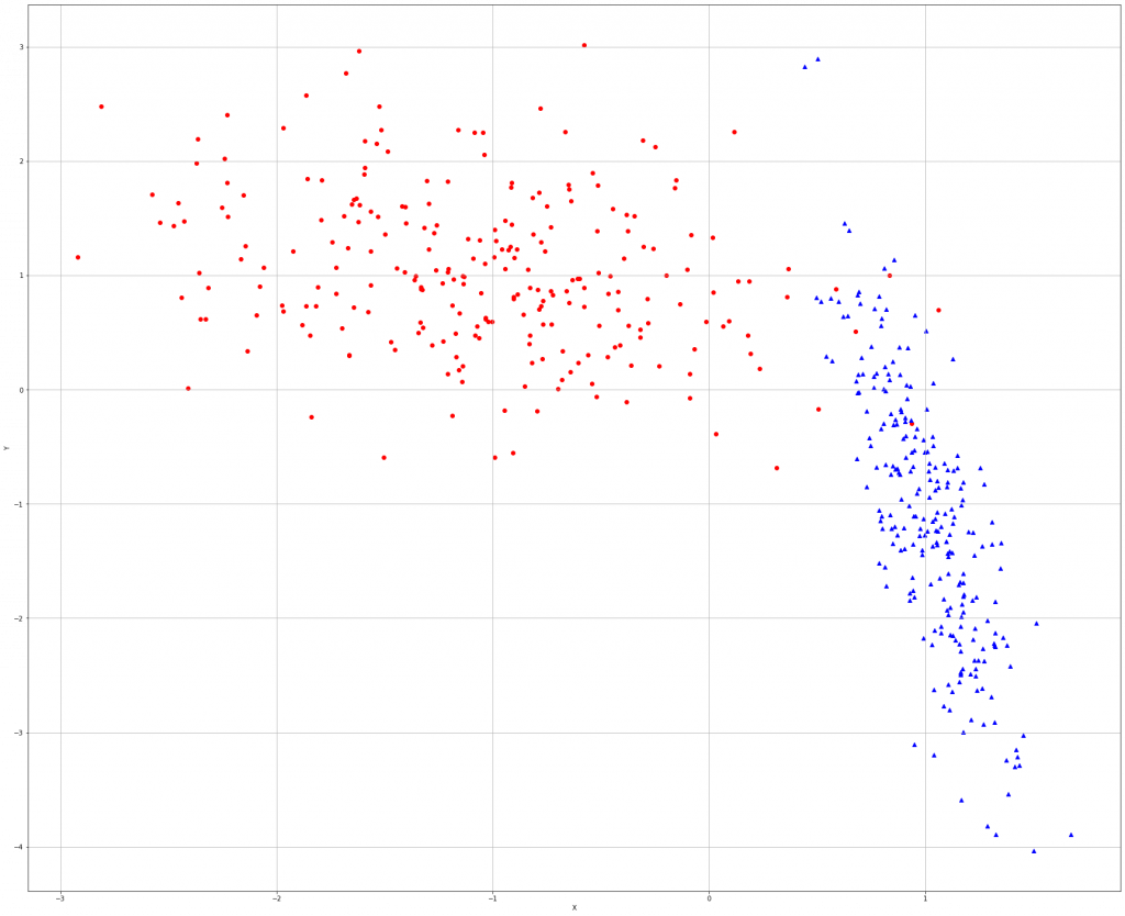
再來，用seed()隨機產生整數的亂數後，設定樣本數，圖中圓點屬於類別0，三角形屬於類別1。

np.random.seed(1000)
nb_samples = 500
def show_dataset(X, Y):
    fig, ax = plt.subplots(1, 1, figsize=(30, 25))

    ax.grid()
    ax.set_xlabel('X')
    ax.set_ylabel('Y')

    for i in range(nb_samples):
        if Y[i] == 0:
            ax.scatter(X[i, 0], X[i, 1], marker='o', color='r')
        else:
            ax.scatter(X[i, 0], X[i, 1], marker='^', color='b')

    plt.show()
    
X, Y = make_classification(n_samples=nb_samples, n_features=2, n_informative=2, n_redundant=0,n_clusters_per_class=1)
show_dataset(X, Y)

接著，與線性迴歸一樣，將資料切分成訓練用及測試用，建模並訓練後，計算準確率，也順便用交叉驗證看看結果。

from sklearn.model_selection import train_test_split
from sklearn.linear_model import LogisticRegression
X_train, X_test, Y_train, Y_test = train_test_split(X, Y, test_size=0.25)
lr = LogisticRegression()
lr.fit(X_train, Y_train)
print('Logistic regression score: %.3f' % lr.score(X_test, Y_test)) // Logistic regression score: 0.992
lr_scores = cross_val_score(lr, X, Y, scoring='accuracy', cv=10)
print('Logistic regression CV average score: %.3f' % lr_scores.mean()) // Logistic regression CV average score: 0.982

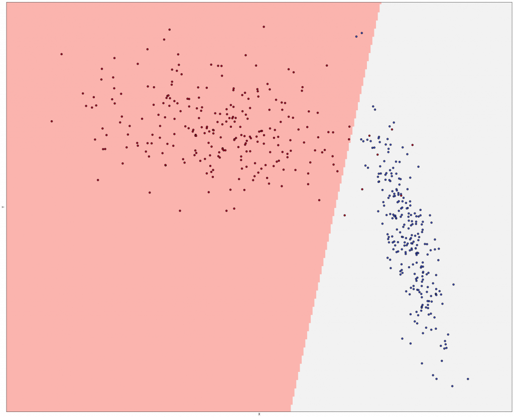
最後，將超平面(一條線)展示出來，順利分成兩群了!!

def show_classification_areas(X, Y, lr):
    x_min, x_max = X[:, 0].min() - .5, X[:, 0].max() + .5
    y_min, y_max = X[:, 1].min() - .5, X[:, 1].max() + .5
    xx, yy = np.meshgrid(np.arange(x_min, x_max, 0.02), np.arange(y_min, y_max, 0.02))
    Z = lr.predict(np.c_[xx.ravel(), yy.ravel()])

    Z = Z.reshape(xx.shape)
    plt.figure(1, figsize=(30, 25))
    plt.pcolormesh(xx, yy, Z, cmap=plt.cm.Pastel1)

    plt.scatter(X[:, 0], X[:, 1], c=np.abs(Y - 1), edgecolors='k', cmap=plt.cm.coolwarm)
    plt.xlabel('X')
    plt.ylabel('Y')

    plt.xlim(xx.min(), xx.max())
    plt.ylim(yy.min(), yy.max())
    plt.xticks(())
    plt.yticks(())

    plt.show()
    
show_classification_areas(X, Y, lr)

隨機梯度下降演算法

Perception(感知器)與Logistic Regression不同在於輸出函數與訓練模型，Perception通常用來最小化實際與預測值之間均方差，Perception只能處理線性問題。
第一步跟之前一樣，先導入資料

from sklearn.datasets import make_classification
nb_samples = 500
X, Y = make_classification(n_samples=nb_samples, n_features=2, n_informative=2, n_redundant=0,n_clusters_per_class=1)

以下就是使用SGD及計算交叉驗證的結果，跟之前的差不多。

sgd = SGDClassifier(loss='perceptron', learning_rate='optimal', n_iter=10)
sgd_scores = cross_val_score(sgd, X, Y, scoring='accuracy', cv=10)
print('Perceptron CV average score: %.3f' % sgd_scores.mean()) // Perceptron CV average score: 0.980

Perception優點：

• 最簡單的線性分類演算法，可推廣至其他複雜的演算法

Perception缺點：

• 一定要線性可分才會停下來（實務上我們沒辦法事先知道資料是否線性可分）

• 錯誤率不會逐步收斂

• 只知道結果是A類還B類，但沒辦法知道是A, B類的機率是多少