Chap.II Machine Learning 機器學習

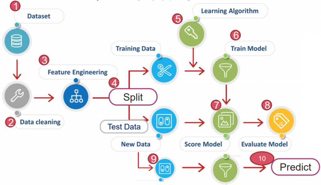
https://yourfreetemplates.com/free-machine-learning-diagram/

Part 3. Learning Algorithm 演算法

本篇會著重在先前提過的監督式學習上。
依據資料類型不同，監督式學習又分以下兩種：

Classification 分類

資料集以＂有限的類別＂分布，對於其做歸類，即分類。

Regresssion 迴歸

資料集以＂連續的方式分布＂，對於其以線性方式描述，即迴歸。

3-1. Weak Learning 弱學習器

概念是由 Michael Kearns 提出，指一個訓練模型結果只比隨機分類好一點的演算法，稱弱學習器。
反之，強學習器則是指經演算法訓練後，模型預測結果非常接近真實情況。

以下會以 breast_cancer（Classification）資料來介紹常見的弱學習器：

import pandas as pd
from sklearn import datasets

ds = datasets.load_breast_cancer()
X=pd.DataFrame(ds.data, columns=ds.feature_names)
y=pd.DataFrame(ds.target, columns=['Cancer'])

from sklearn.model_selection import train_test_split
X_train, X_test, y_train, y_test = train_test_split(X, y, test_size = 0.3)

from sklearn.preprocessing import StandardScaler
sc = StandardScaler()
X_train_std = sc.fit_transform(X_train)
X_test_std = sc.fit_transform(X_test)

A. K-Nearest Neighbors (KNN) 最近距離法

尋找距離預測值最近的 N 個樣本點，以多數決（Majority Voting）決定所屬分類。

優點：實現只須兩個參數 P & 距離函數。
缺點：無法應用於高維度，且不適用類別（定性）特徵（如性別、星期幾...等非數字資料）。
常用於推薦商品。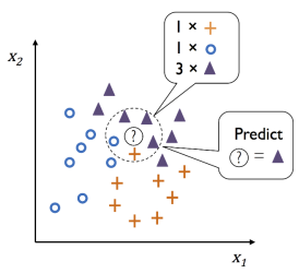

from sklearn.neighbors import KNeighborsClassifier as knn
clf = KNN(n_neighbors = 3)
clf.fit(X_train_std, y_train)

clf.score(X_test, y_test)
>>  0.9707602339181286

超參數：
1. n_neighbors: 預測值須取多少臨近點比較。為避免平局常取奇數。
2. metric: 計算距離的公式。

B. Logistic Regresssion 羅吉斯迴歸

其為線性迴歸的改良版。（數學原理可參考：推導1、推導2 & 推導3）

優點：Outlier 影響小（上下限 0~1），可線性分割。平滑曲線，變異性小。
缺點：無法應用於高維度、易未擬合，且對於非線性特徵要額外轉換。
常用於二分類。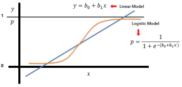

from sklearn.linear_model import LogisticRegression as LR
clf = LR(penalty='l2', C=0.01)
clf.fit(X_train_std, y_train)

clf.score(X_test_std, y_test)

>>  0.9649122807017544

超參數：
1. penalty: 正則化參數。預設 l2。（詳細解說）
L1: 將沒有用的權重設為0，留下模型認為重要的權重
L2: 削弱所有權重（但仍保留），讓所有權重與神經元都處於活動狀態。
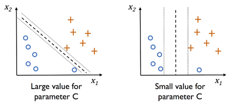
2. C: 正則化強度的倒數。C 越小，矯正強度越大（使訓練分數降低、預測資料變準）。

C. Support Vector Machine 支援向量機（SVM）

如圖，距離 model（方程式）最近的點，稱為 Support Vector 支援向量，
而 positive Hyperplane & negative Hyperplane 彼此間距為 margin。
其根本目的為找到一個 Decision Boundary，使切割的 margin 越大越好。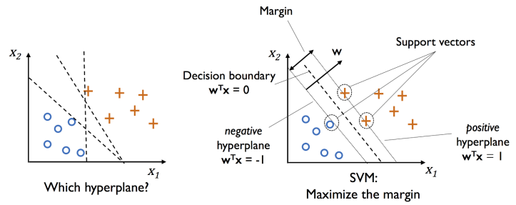

優點：Outlier 影響小（僅邊界影響），且記憶體用量小。高維資料表現好。多樣核函數以應對資料。
缺點：樣本數大時效能差（須來回優化），成本貴。

from sklearn.svm import SVC
clf = SVC(C=1, probability=True)
clf.fit(X_train_std, y_train)

clf.score(X_test_std, y_test)

>>  0.9649122807017544

可以查看其參照多少支援向量：

len(clf.support_vectors_)

>>  97

超參數：
1. C: 正則化強度的倒數。C 越小，矯正強度越大（使訓練分數降低、預測資料變準）。
默認 1（hard margin，盡可能找出完美超平面，下圖左）。
若 C=0.01，則模型評分會下降至 0.66。

2. kernel: 同 PCA，有 {‘linear’, ‘poly’, ‘rbf’, ‘sigmoid’, ‘precomputed’} 等分類方式。
若使用 'linear' 分析圓形資料，評分會下降許多
3. probability: True 才能使用 predict_proba 呼叫機率。

PS. 此外，sklearn 有提供三種線性分類寫法：

# 1. 較常使用
LinearSVC(C=1, loss='hinge')

# 2. 執行效能較差
SVC(kernal='linear', C=1)

# 3. 適合記憶體有限（訓練資料很龐大） or Online Training
SGDClassifier(loss='hinge', alpha=1/(m*C))

D. Decision Tree 決策樹

透過 training data 的 fearture 學出一系列的問題，然後來推斷其分類。

演算法
A. Sklearn 使用的是 Classification and Regression Tree (CART)
特色為依照數值型特徵切割，且一次切割只分為兩個點，但同一特徵可多次切割。
B. Chi-squared Automatic Interaction Detection (CHAID)
所有變數轉成不連續的組距（discretecized），切割可大於兩個點。
C. 其他還有 ID3、ID4.5、ID5.0、Decision Stump、M5...等。

Information gain 信息增益
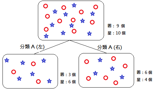
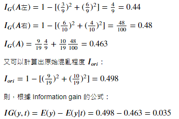
為了能在節點上使用最具意義的特徵來分割，我們會透過信息增益來判斷。
信息增益越大，那此「分類」對於決策樹來說就越重要，表示它能把數據分的越乾淨。
所謂的信息增益，可用以下方式表達：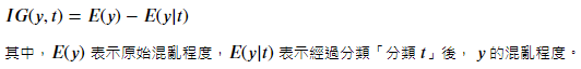

常見信息增益計算：
A. Gini Impurity 吉尼不純度：
計算一「隨機樣本」被某個「分類 x 」分錯的概率。不純度越低，表示該分類方法越顯著有用。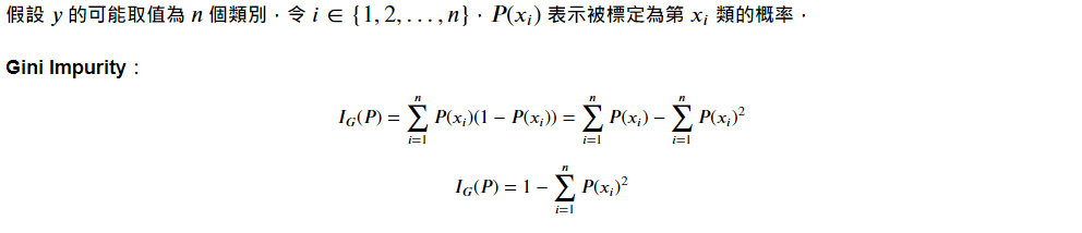

Ex. 假設分類後僅剩下 1 種特徵，則 Ig = 1-(1+0) = 0，為一個不純度最低的完美分類方法。
（多考慮純度，故比起 Entropy，分類效果較好）

B. Entropy 熵：
類似熱力學，但在資訊理論中多了負號。熵高（負少）傳輸資訊多，熵低（負多）則傳輸資訊少。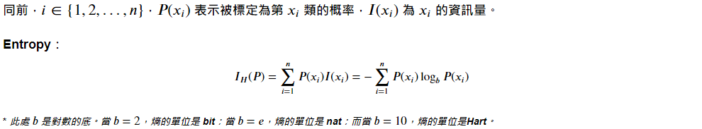

C. Classification Error 分類錯誤率：
很直觀，即分類錯誤的最小機率。

優點：易於瞭解與解釋（可視覺化）。資料僅須少量前處理（不需常態/標準化）。無複雜計算。
缺點：易過擬合，需搭配特徵選擇減少特徵量。不平衡樣本（得病/無病）差距太多，會使分割偏向多數樣本方，需使用 class balancing 技術（如 SMOTE）矯正。

程式碼
*注意!!! 決策樹演算不需要標準化/正則化的!!!
它們不關心特徵「值」，只關心特徵「分佈」和特徵間的「條件概率」

import pandas as pd
from sklearn import datasets

ds = datasets.load_breast_cancer()
X=pd.DataFrame(ds.data, columns=ds.feature_names)
y=pd.DataFrame(ds.target, columns=['Cancer'])

from sklearn.model_selection import train_test_split
X_train, X_test, y_train, y_test = train_test_split(X, y, test_size = 0.3)

決策樹：

from sklearn.tree import DecisionTreeClassifier as DTC
clf = DTC(criterion='gini', max_depth=3, random_state=1)
clf.fit(X_train, y_train)

clf.score(X_test, y_test)

>>  0.9064327485380117

超參數：
1. criterion: 不純度方法，'gini'（默認） & 'entropy'。
2. max_depth: 樹的層數。若 None 則擴展節點至所有葉包含 min_samples_split 樣本。默認 None。
3. min_samples_split: 分裂一個內部節點所需的最小樣本數。默認 2。
更多參數看 DecisionTreeClassifier或 DecisionTreeRegressor

要讓決策樹視覺化，需安裝以下兩個程式：

1. Graphviz (官方網站)
   下載後，進入主機（右鍵）內容 -> 進階系統設定 -> 環境變數 -> Path
   並新增＂C:\Users\User.conda\envs\tensorflow-gpu\Lib\site-packages\graphviz\bin＂

2. 使用 pip 安裝 pydotplus

pip install pydotplus

正式使用：

# 作圖
from pydotplus import graph_from_dot_data
from sklearn.tree import export_graphviz

dot_data = export_graphviz(clf,
                          filled = True,
                          class_names = ds.target_names,
                          feature_names = ds.feature_names,
                          out_file = None)
graph = graph_from_dot_data(dot_data)
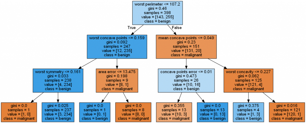
graph.write_png('Pic\Cancer tree.png')

# 顯示圖片
from IPython.display import Image
Image(filename='Pic\Cancer tree.png', width=1000)

另外，Decision Tree 也可以應用於迴歸類型的資料，見補充 4.。

結論：

1. KNN: 實現僅需兩參數。但高維表現弱。可用於推薦商品。
2. Logistic Regresssion: 以 0~1 分割資料。但高維表現差。可用於二分法演算。
3. SVM: 邊界影響小，高維表現好，可分析多種類型（如圓球形）資料。但耗時長成本高。
4. Decision Tree: 可視覺化，資料不需前處理。但易過擬合，且若樣本差距過大需矯正。
5. Random Forest: 高維表現好，能平衡資料誤差。但記憶體消耗高，且無法針對單一樹解釋。
   .
   .
   .
   .
   .
   *補充 1.：Gini Impurity
   
   

*補充 2.：Entropy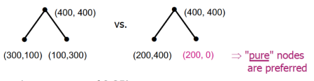

左右兩邊的 Etropy 算出來皆為 0.5，但

*補充 3.：客戶留存率與流失率

*補充 4.：Decision Tree 迴歸 Boston

from sklearn.datasets import load_boston
from sklearn.tree import DecisionTreeRegressor as DTR
import pandas as pd

ds = load_boston()
X=pd.DataFrame(ds.data, columns=ds.feature_names)
y=pd.DataFrame(ds.target, columns=['Boston'])

from sklearn.model_selection import train_test_split
X_train, X_test, y_train, y_test = train_test_split(X, y, test_size = 0.3)

clf = DTR(max_depth=2, random_state=1)
clf.fit(X_train, y_train)
clf.score(X_test, y_test)

>>  0.6865210494380858

.
.
.
.
.

Homework Answer：

試著用 sklearn 的資料集 breast_cancer，操作 Featuring Extraction (by PCA)。

# Datasets
from sklearn.datasets import load_breast_cancer
import pandas as pd

ds = load_breast_cancer()

df_X = pd.DataFrame(ds.data, columns=ds.feature_names)
df_y = pd.DataFrame(ds.target, columns=['Cancer or Not'])

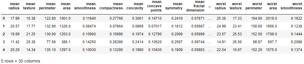
df_X.head()

# define y
df_y['Cancer or Not'].unique()

>>  array([0, 1])

# Split
from sklearn.model_selection import train_test_split

X_train, X_test, y_train, y_test = train_test_split(df_X, df_y, test_size=0.3)
X_train.shape, X_test.shape

>>  ((398, 30), (171, 30))

from sklearn.decomposition import PCA

pca1 = PCA(n_components=2)
X_train_pca = pca1.fit_transform(X_train)
X_test_pca = pca1.transform(X_test)

X_train_pca.shape, X_test_pca.shape

>>  ((398, 2), (171, 2))

# Modeling (by LogisticRegression)
from sklearn.linear_model import LogisticRegression as lr

clf = lr(solver='liblinear')
clf.fit(X_train_pca, y_train)

print(clf.score(X_test_pca, y_test))

>>  0.9298245614035088