Hi! 大家好，我是Eric，這次要來用Python做決策樹。

• 緣起：決策樹因為相對於其他機器學習模型而言，是較易被解釋的，所以是蠻常見的分類方法。
• 方法：運用 [Python]的[sklearn的tree.DecisionTreeClassifier] 套件。
• 使用資料：kaggle的加州警備隊(SWITRS)提供的加州交通事故資料集(collisions)。
• 參考來源：
• https://www.kaggle.com/alexgude/california-traffic-collision-data-from-switrs

0. 在使用python前，由於電腦硬體本身限制，故先以EmEditor軟體做初步的篩選，將資料量大幅減少，再輸入到python中。

1. 載入套件及初步篩選出欲使用的資料。

# 載入資料
import pandas as pd
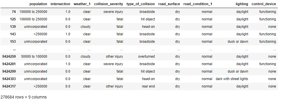
cm = pd.read_csv('colli_motor.txt', sep=",")

# 篩選資料，篩選出與機車有關的資料
cm_mot = cm[cm["motorcycle_collision"] == 1]
cm_mot_d = cm_mot.drop("motorcycle_collision", axis=1)

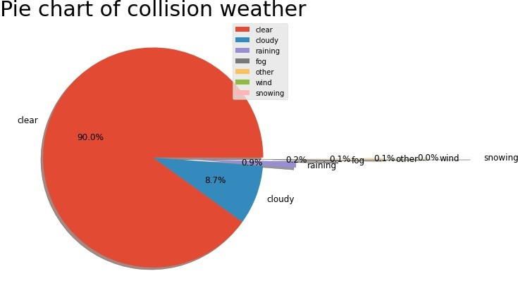
2. 敘述性分析，先查看變數的資料值比例。

# 各變數資料圓餅圖-以天氣變數為例，其於變數作法相同

import matplotlib.pyplot as plt 

weather = cm_mot_d["weather_1"].value_counts() 
weather
weather2 = weather.to_frame(name = "count")
print(weather2)
weather2.insert(0, column="weather", value=["clear", "cloudy", "raining", "fog", "other", "wind", "snowing"])
print(weather2)

plt.figure(figsize=(7,10))    # 顯示圖框架大小

labels = weather2["weather"]      # 製作圓餅圖的類別標籤
separeted = (0, 0, 0.3, 0.7, 1.1, 1.5, 1.9)                  # 依據類別數量，分別設定要突出的區塊
size = weather2["count"]                         # 製作圓餅圖的數值來源

plt.pie(size,                           # 數值
        labels = labels,                # 標籤
        autopct = "%1.1f%%",            # 將數值百分比並留到小數點一位
        explode = separeted,            # 設定分隔的區塊位置
        pctdistance = 0.6,              # 數字距圓心的距離
        textprops = {"fontsize" : 12},  # 文字大小
        shadow=True)                    # 設定陰影

 
                                         # 使圓餅圖比例相等
plt.title("Pie chart of collision weather", {"fontsize" : 30})  # 設定標題及其文字大小
plt.legend(loc = "best")                                   # 設定圖例及其位置為最佳

plt.savefig("Pie chart of collision weather.jpg",   # 儲存圖檔
            bbox_inches='tight',               # 去除座標軸占用的空間
            pad_inches=0.0)                    # 去除所有白邊
plt.close()      # 關閉圖表

3.1 資料前置處理-檢查Null、NaN值。

#載入資料處理與決策樹分析套件
from sklearn import tree
from sklearn.metrics import confusion_matrix
from sklearn.metrics import classification_report
from sklearn.model_selection import train_test_split
from sklearn import metrics

# 檢查是否有Null與NaN值
import numpy as np

print(np.isnan(cm_mot_d.any()))     #檢查是否有NaN值
print()

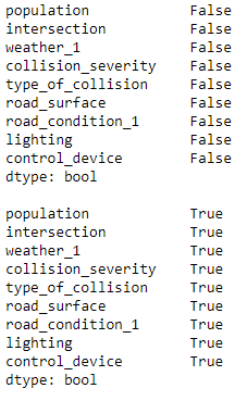
print(np.isfinite(cm_mot_d.all()))  # 檢查資料是否為有限值

cm_mot_d.isnull().sum() #檢查是否有null

#處理有null的欄位，移除null的資料列

cm_mot_d2 = cm_mot_d[cm_mot_d["population"].notnull()]
cm_mot_d3 = cm_mot_d2[cm_mot_d2["intersection"].notnull()]
cm_mot_d4 = cm_mot_d3[cm_mot_d3["weather_1"].notnull()]
cm_mot_d5 = cm_mot_d4[cm_mot_d4["type_of_collision"].notnull()]
cm_mot_d6 = cm_mot_d5[cm_mot_d5["road_surface"].notnull()]
cm_mot_d7 = cm_mot_d6[cm_mot_d6["road_condition_1"].notnull()]
cm_mot_d8 = cm_mot_d7[cm_mot_d7["lighting"].notnull()]
cm_mot_d9 = cm_mot_d8[cm_mot_d8["control_device"].notnull()]
  
print(cm_mot_d9.isnull().any().any())  #再次檢查是否還有null

3.2 資料前置處理-將目標變數轉為二元。

#資料前處理，由於CART是二元，所以將y分成嚴重與不嚴重，嚴重包含fatal、severe injury；不嚴重包含property damage only、pain、other injury

for i in range(len(cm_mot_d9["collision_severity"])):
    if cm_mot_d9["collision_severity"].iloc[i] == "fatal":
        cm_mot_d9["collision_severity"].iloc[i] = "severe"
    elif cm_mot_d9["collision_severity"].iloc[i] == "severe injury":
        cm_mot_d9["collision_severity"].iloc[i] = "severe"
    elif cm_mot_d9["collision_severity"].iloc[i] == "property damage only":
        cm_mot_d9["collision_severity"].iloc[i] = "not severe"
    elif cm_mot_d9["collision_severity"].iloc[i] == "pain":
        cm_mot_d9["collision_severity"].iloc[i] = "not severe"
    else:
        cm_mot_d9["collision_severity"].iloc[i] = "not severe"

3.3 資料前置處理-製作虛擬變數(dummy variable)。

#為了dummy後，other不重複欄位名稱，排除other
cm_mot_d9_2 = cm_mot_d9[cm_mot_d9["type_of_collision"] != "other"]
cm_mot_d9_3 = cm_mot_d9_2[cm_mot_d9_2["weather_1"] != "other"]
cm_mot_d9_4 = cm_mot_d9_3[cm_mot_d9_3["road_condition_1"] != "other"]

#取出X與Y
cm_mot_d9_4_y = cm_mot_d9_4["collision_severity"]
cm_mot_d9_4_X = cm_mot_d9_4.drop("collision_severity", axis=1)

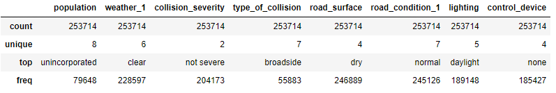
cm_mot_d9_4.describe(include = ["object"]) # 類別資料敘述分析

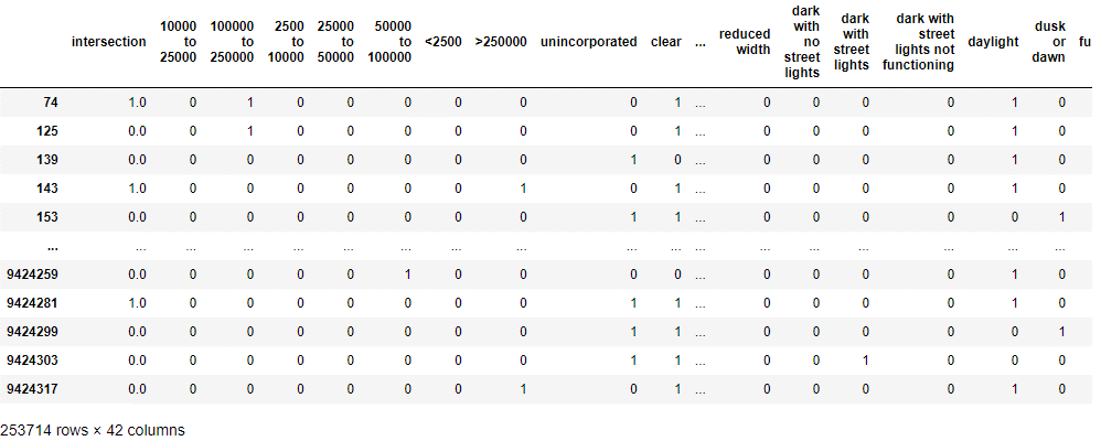
#x資料前處理，轉換為dummy variable使資料符合使用CART (https://towardsdatascience.com/the-dummys-guide-to-creating-dummy-variables-f21faddb1d40)

population2 = pd.get_dummies(cm_mot_d9_4_X["population"])
weather_1_2 = pd.get_dummies(cm_mot_d9_4_X["weather_1"])
type_of_collision2 = pd.get_dummies(cm_mot_d9_4_X["type_of_collision"])
road_surface2 = pd.get_dummies(cm_mot_d9_4_X["road_surface"])
road_condition_1_2 = pd.get_dummies(cm_mot_d9_4_X["road_condition_1"])
lighting2 = pd.get_dummies(cm_mot_d9_4_X["lighting"])
control_device2 = pd.get_dummies(cm_mot_d9_4_X["control_device"])

cm_mot_d9_4_X2 = pd.concat([cm_mot_d9_4_X, population2, weather_1_2, type_of_collision2, road_surface2, road_condition_1_2, lighting2, control_device2], axis=1)
cm_mot_d9_4_X3 = cm_mot_d9_4_X2.drop("population", axis=1)
cm_mot_d9_4_X4 = cm_mot_d9_4_X3.drop("weather_1", axis=1)
cm_mot_d9_4_X5 = cm_mot_d9_4_X4.drop("type_of_collision", axis=1)
cm_mot_d9_4_X6 = cm_mot_d9_4_X5.drop("road_surface", axis=1)
cm_mot_d9_4_X7 = cm_mot_d9_4_X6.drop("road_condition_1", axis=1)
cm_mot_d9_4_X8 = cm_mot_d9_4_X7.drop("lighting", axis=1)
cm_mot_d9_4_X9 = cm_mot_d9_4_X8.drop("control_device", axis=1)

4. 建立決策樹模型。

# 切分訓練與測試資料
train_X, test_X, train_y, test_y = train_test_split(cm_mot_d9_4_X9, cm_mot_d9_4_y, test_size = 0.3)

#先查看不同深度的準確度，以決定
# List of values to try for max_depth:
max_depth_range = list(range(3, 13))
# List to store the accuracy for each value of max_depth:
accuracy = []
for depth in max_depth_range:
    clf = tree.DecisionTreeClassifier(criterion="gini", max_depth = depth)
    clf.fit(train_X, train_y)
    test_y_predicted = clf.predict(test_X)
    score = metrics.accuracy_score(test_y, test_y_predicted)
    accuracy.append(score)
    
print(accuracy)

#查看不同子節點最小樣本數的準確度
# List of values to try for max_depth:
min_leaf_range = list(range(5, 15))
# List to store the accuracy for each value of max_depth:
accuracy = []
for leaf in min_leaf_range:
    clf2 = tree.DecisionTreeClassifier(criterion="gini", max_depth = 3, min_samples_leaf = leaf)
    clf2.fit(train_X, train_y) 
    test_y_predicted2 = clf2.predict(test_X)
    score = metrics.accuracy_score(test_y, test_y_predicted2)
    accuracy.append(score)
    
print(accuracy)

# 建立分類器 (http://www.taroballz.com/2019/05/15/ML_decision_tree_detail/)
clf3 = tree.DecisionTreeClassifier(criterion="gini", max_depth = 3)
clf3.fit(train_X, train_y)

# 預測
test_y_predicted3 = clf3.predict(test_X)

# 績效
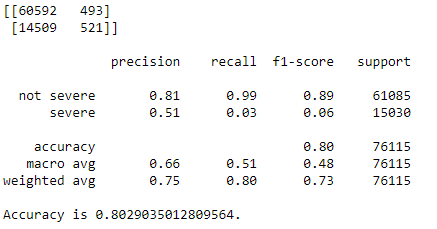
print(confusion_matrix(test_y, test_y_predicted3))
print() 
print(classification_report(test_y, test_y_predicted3))
accuracy = metrics.accuracy_score(test_y, test_y_predicted3)
print(f"Accuracy is {accuracy}.")

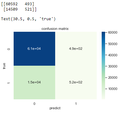
# 製作混淆矩陣熱力圖
import seaborn as sns

sns.set()
f,ax=plt.subplots()
C2= confusion_matrix(test_y, test_y_predicted3, labels = ["not severe", "severe"])
print(C2) #打印出來看看
sns.heatmap(C2, annot=True, ax=ax, cmap = "GnBu") #畫熱力圖

ax.set_title('confusion matrix') #標題
ax.set_xlabel('predict') #x軸
ax.set_ylabel('true') #y軸

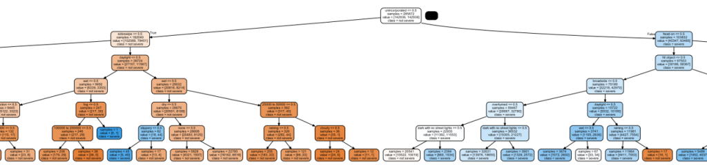
5. 視覺化。

features = list(cm_mot_d9_4_X9[:])


# viz code

from six import StringIO
import pydot
import pydotplus


dot_data = StringIO()
tree.export_graphviz(clf3,
        out_file=dot_data,
        feature_names=features,
        class_names=clf3.classes_,
        filled=True, rounded=True,
        impurity=False)

graph = pydotplus.graph_from_dot_data(dot_data.getvalue())
graph.write_pdf("cm7.pdf")

6. 大功告成。
運用CART的重點有：1.將目標變數轉為二元化。2.將自變數轉為虛擬變數。