為何需要處理不平衡資料

在進行分類問題時，可能會碰到資料不平衡的問題。人們往往會透過模型想要找到數據中較為少數的那部分，如：信用卡盜刷紀錄、垃圾郵件識別等。當數據出現不平衡時，若模型在測試資料集中皆預測為人數較多的那個類別時，雖然可以達到較高的準確率，但並不代表此模型能夠準確幫助分類，因此在資料內數量比例超過1:4時，就建議在分析前將資料不平衡的問題納入考量。

處理不平衡資料

在處理不平衡資料時，可考量使用以下幾種作法：

1. 使用準確率以外的衡量變量:
   如：精確度/召回率、F1 score等，而不再依靠準確率來作為主要的模型衡量指標

2. Oversampling:
   將樣本數較少的組別之數據隨機選取並進行複製，使得各組之間的數據量可以達到相同，但若將同樣的數據複製多份，可能會導致模型會出現過度擬合(Overfitting)的問題。

3. SMOTE(Synthetic Minority Over-sampling Technique)：
   合成少數過採樣方法，為random oversampling改進後的方法，概念是對少數類的樣本進行分析，並人工合成新樣本添加到數據集中。由於此方法並不會考量其他樣本的情況，因此若所選取的少樣類樣本周遭皆是多數類別的樣本，則所選取到的樣本可能就是噪音，使得新合成的樣本會與多數樣本產生重疊，進而導致模型分類的困難。

4. Undersampling:
   在樣本數較多的組別中，隨機挑選若干筆數據，使各組的數據量達到相同。此方法會丟失許多訊息，因此延伸出多個方法來減少過多的訊息量損失，如：使用Ensemble learning的方法(EasyEnsemble, BalanceCascade, NearMiss)來改善隨機抽樣導致重要樣本被刪除的問題。

5. 調整使用的演算法
   在使用的模型/演算法中將各個類別的資料數量納入考量，透過權重進行調整，此概念稱為成本敏感學習技術(Cost-Sensitive Learning)。舉例：在訓練決策樹(decision tree)時，可以設定不同權重給予不同類別，使得在訓練時，可以改善資料不平衡所遇到的問題。

在進行資料分析時，不平衡的問題常會出現，如：醫學資料中患有疾病與健康受試者常常就會出現不平衡的問題，因此此議題仍是非常重要的。
由於本次使用的資料集包含的是時序資料，而時序資料的imbalance問題有許多更加深入的處理方法，因此在本次實作中將採用模擬資料來做示範。

實作

產生模擬資料

R:

set.seed(2022) ### 設定隨機種子，使每次產生的資料相同

n1 <- 200 # 第一類的數量(type1)
n2 <- 20  # 第二類的數量(type2)

## 產生type1的data 
x <- rnorm(mean = 0, sd = 0.5, n = n1)
y <- rnorm(mean = 0, sd = 1, n = n1)
data1 <- data.frame(label=rep("type1", n1),x=x, y=y, stringsAsFactors = T)

## 產生type2的data 
x2 <- rnorm(mean = 2, sd = 0.5, n = n2)
y2 <- rnorm(mean = 2, sd = 1, n = n2)
data2 <- data.frame(label=rep("type2", n2), x=x2, y=y2, stringsAsFactors = T)

## 建立 imbalanced_data
imbalanced_data <- rbind(data1, data2)
table(imbalanced_data$label)
#type1 type2 
#  200    20 

Python:

import random
import numpy as np
import pandas as pd

### 設定隨機種子，使每次產生的資料相同
random.seed(2022)

n1 = 200 # 第一類的數量(type1)
n2 = 20  # 第二類的數量(type2)

## 產生type1的data 
x = np.random.normal(0,0.5,n1)
y = np.random.normal(0,1,n1)
data1 = pd.DataFrame({'label':['type1']*n1,'x':x,'y':y})

## 產生type2的data 
x2 = np.random.normal(2,0.5,n2)
y2 = np.random.normal(2,1,n2)
data2 = pd.DataFrame({'label':['type2']*n2,'x':x2,'y':y2})

## 建立 imbalanced_data
imbalance_data = pd.concat([data1, data2])
imbalance_data['label'].value_counts()
#type1    200
#type2     20

Random Oversampling

R:

## 在較少數的類別(type2)中，隨機抽樣取後放回，產生新的資料點
new_data <- data2[sample(nrow(data2), size = n1-n2, replace = T),]
balanced_data <- rbind(imbalanced_data, new_data)
table(balanced_data$label)
#type1 type2 
#  200   200

## 繪圖
library(ggplot2)
library(ggpubr) 
p1 <- ggplot(data = imbalanced_data,aes(x=x,y=y,colour=label))+
  geom_point()+
  ggtitle("Imbalance data")
p2 <- ggplot(data = balanced_data,aes(x=x,y=y,colour=label))+
  geom_point()+
  ggtitle("Balanced data(Oversampling)")
ggarrange(p1,p2, ncol = 2,nrow = 1,common.legend = T,legend="bottom")

Random Oversampling所產生的點會和原始資料點重疊！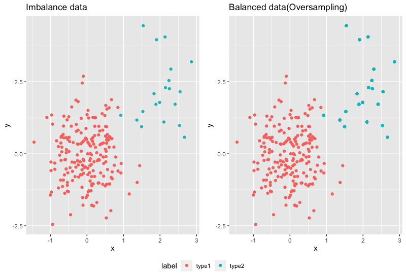

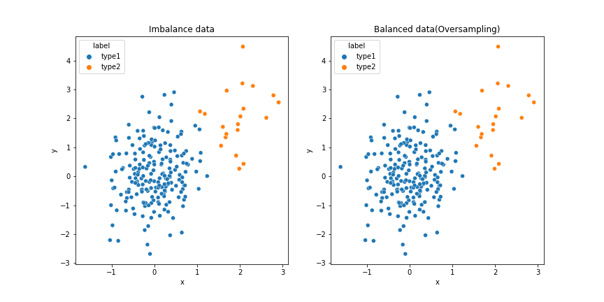
Python: 使用imblearn.over_sampling套件中的RandomOverSampler

import imblearn
from imblearn.over_sampling import RandomOverSampler
from collections import Counter

oversample = RandomOverSampler(sampling_strategy='minority')
X_over, y_over = oversample.fit_resample(imbalance_data[['x','y']], imbalance_data['label'])

balanced_data = X_over
balanced_data['label'] = label
print(Counter(balanced_data['label'] ))
# Counter({'type1': 200, 'type2': 200})

##繪圖
import seaborn as sns
import matplotlib.pyplot as plt

sns.scatterplot(data=imbalance_data, x='x', y='y', hue='label',ax=axs[0]).set(title='Imbalance data')
sns.scatterplot(data=balance_data, x='x', y='y', hue='label',ax=axs[1]).set(title='Balanced data(Oversampling)')

SMOTE

R: 使用performanceEstimation套件的smote語法

library(performanceEstimation)
## default: smote(form, data, perc.over = 2, k = 5, perc.under = 2)
## perc.over: 控制minority class進行over-sampling
## perc.under: 控制majority classes進行under-sampling
newData <- smote(label ~ .,imbalanced_data, perc.over = 4)
table(newData$label)
#type1 type2 
#  160   100 

## 繪圖
p3 <- ggplot(data = newData,aes(x=x,y=y,colour=label))+
  geom_point()+
  ggtitle("Balanced data(SMOTE)")
ggarrange(p1,p3, ncol = 2,nrow = 1,common.legend = T,legend="bottom")

Python: 使用imblearn.over_sampling套件中的SMOTE

from imblearn.over_sampling import SMOTE

X_smote, label = SMOTE(random_state=2022).fit_resample(imbalance_data[['x','y']], imbalance_data['label'])

newData = X_smote
newData['label'] = label
print(Counter(newData['label'] ))
#Counter({'type1': 200, 'type2': 200})

##繪圖
fig, axs = plt.subplots(ncols=2,figsize=(12, 6))

sns.scatterplot(data=imbalance_data, x='x', y='y', hue='label',ax=axs[0]).set(title='Imbalance data')
sns.scatterplot(data=newData, x='x', y='y', hue='label',ax=axs[1]).set(title='Balanced data(SMOTE)')

Undersampling

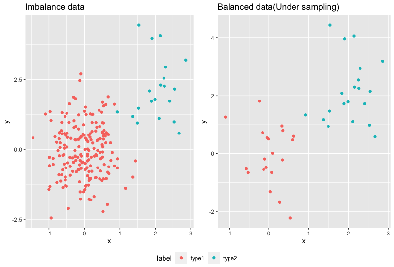
R:使用ROSE套件，ovun.sample語法

library(ROSE)]
# 設定method為'under', N的數量為minority class的兩倍
balanced_sample  <-ovun.sample(label ~ ., data = imbalanced_data, method = "under", N=n2*2, seed = 5)$data
table(balanced_sample$label)
#type1 type2 
#   20    20

## 繪圖
p3 <- ggplot(data = newData,aes(x=x,y=y,colour=label))+
  geom_point()+
  ggtitle("Balanced data(SMOTE)")
ggarrange(p1,p3, ncol = 2,nrow = 1,common.legend = T,legend="bottom")

Python: 使用imblearn.under_sampling套件中的RandomUnderSampler

from imblearn.under_sampling import RandomUnderSampler

oversample = RandomUnderSampler(sampling_strategy='majority')
X_under, label = oversample.fit_resample(imbalance_data[['x','y']], imbalance_data['label'])

balanced_sample = X_under
balanced_sample['label'] = label
print(Counter(balanced_sample['label'] ))
# Counter({'type1': 20, 'type2': 20})

##繪圖
fig, axs = plt.subplots(ncols=2,figsize=(12, 6))

sns.scatterplot(data=imbalance_data, x='x', y='y', hue='label',ax=axs[0]).set(title='Imbalance data')
sns.scatterplot(data=balanced_sample, x='x', y='y', hue='label',ax=axs[1]).set(title='Balanced data(Under sampling)')