As I find out it's easier to type in Eng rather than switch the languages while I writing the articles.

Thus, I feel like to keep typing in Eng again ahaha, plz forgive me that I can't be bother to type in Mandarin lalala... ~ ~ ~

Introduction:

As stated earlier, ARIMA(p,d,q) are one of the most popular econometrics models used to predict time series data such as stock prices, demand forecasting, and even the spread of infectious diseases.

An ARIMA model is basically an ARMA model fitted on d-th order differenced time series such that the final differenced time series is stationary.

A stationary time series is one whose statistical properties such as mean, variance, autocorrelation, etc. are all constant over time.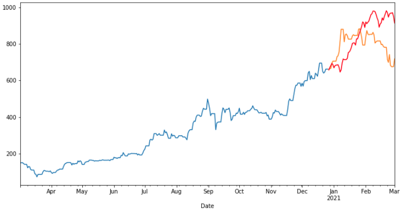

What is "ARIMA" ?

ARIMA stands for AutoRegressive Integrated Moving Average

AutoRegressive Model (AR)

Auto Regressive Model forecast the values based on past values that have effect on current value. If we are about to forecast a monthly sales, then sales of November depends on sales of October, September and soon.

Integrated (I)

Time Series are stationary if the mean and variance is consistent over time. This happens only if they donot have trend or seasonal effects. A stationarized series is relatively easy to predict because of constant stationary terms

Moving Average Model (MA)

Moving Average model forecast the values based on previous days error terms that have effect on current value.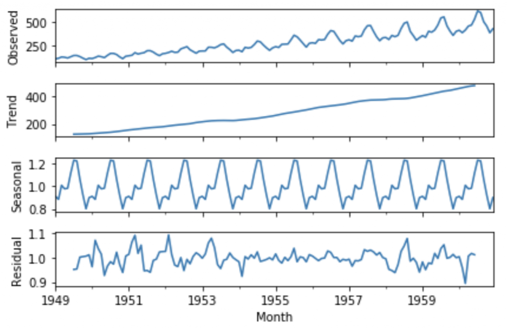

Pros & Cons of ARIMA:

Pros of ARIMA models

• Only requires the prior data of a time series to generalize the forecast.
• Performs well on short term forecasts.
• Models non-stationary time series.

Cons of using ARIMA models

• Difficult to predict turning points.
• There is quite a bit of subjectivity involved in determining (p,d,q) order of the model.
• Computationally expensive.
• Poorer performance for long term forecasts.
• Cannot be used for seasonal time series.
• Less explainable than exponential smoothing.

An experimental study of ARIMA:

*Notice: You can print out the result by each step. Run the xxx.py for checkinig your code :)
*The dataset needs to have a column that contains date or time, as it needs a period of time's (Regression) dataset for the prediction. Good Luck! :)

Step 1. import the packages:

Example dataset: Click ME !
Don't forget to do pip install pyramid-arima in Pycharm terminal, before you start the programing.

# coding: utf-8
import numpy as np 
import pandas as pd 
import sklearn
from statsmodels.graphics.tsaplots import plot_acf, plot_pacf
import matplotlib.pyplot as plt
import statsmodels.api as sm
from statsmodels.tsa.arima_model import ARIMA

Step 2. Prepare the data

Example dataset: Click ME !

df = pd.read_csv('usa_date.csv')
print(df)

Step 3. Precise / Prepare the data

## 決定訓練/測試數據要用的區間
## filter data after 2021-12
df = df['id']
df_train = df.iloc[328:449]
df_test = df.iloc[449:478]
#訓練數據整理
df_order= df_train.reset_index(drop=True)

Step 4. Draw the graphs

## acf plot 
plt.rcParams.update({'figure.figsize':(9,7), 'figure.dpi':120})
# Import data : Internet Usage per Minute
df = df_order
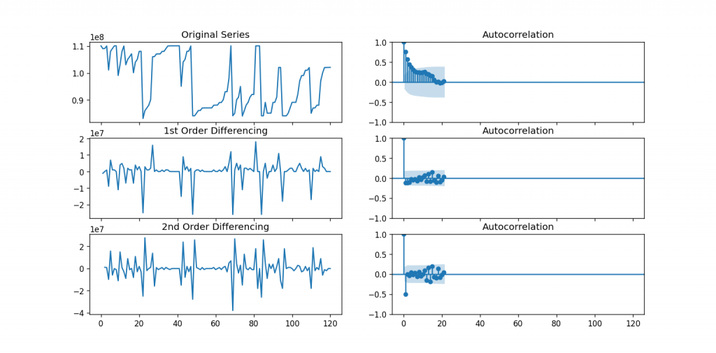
# Original Series
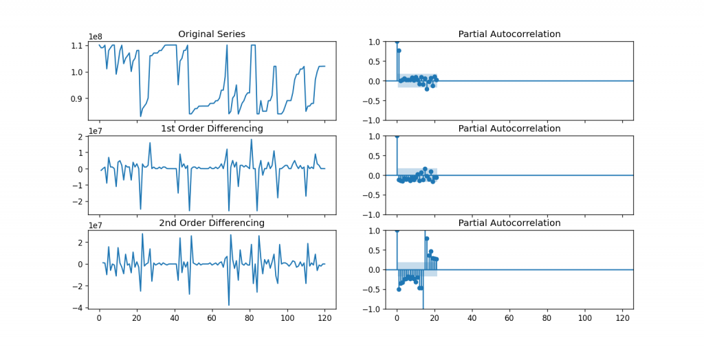
fig, axes = plt.subplots(3, 2, sharex=True)
axes[0, 0].plot(df_order); axes[0, 0].set_title('Original Series')
plot_acf(df_order, ax=axes[0, 1])

# 1st Differencing
axes[1, 0].plot(df_order.diff()); axes[1, 0].set_title('1st Order Differencing')
plot_acf(df_order.diff().dropna(), ax=axes[1, 1])
# 2nd Differencing
axes[2, 0].plot(df_order.diff().diff()); axes[2, 0].set_title('2nd Order Differencing')
plot_acf(df_order.diff().diff().dropna(), ax=axes[2, 1])
plt.show()
## pacf plot # Original Series
fig, axes = plt.subplots(3, 2, sharex=True)
axes[0, 0].plot(df_order); axes[0, 0].set_title('Original Series')
plot_pacf(df_order, ax=axes[0, 1])

# 1st Differencing
axes[1, 0].plot(df_order.diff()); axes[1, 0].set_title('1st Order Differencing')
plot_pacf(df_order.diff().dropna(), ax=axes[1, 1])
# 2nd Differencing
axes[2, 0].plot(df_order.diff().diff()); axes[2, 0].set_title('2nd Order Differencing')
plot_pacf(df_order.diff().diff().dropna(), ax=axes[2, 1])
plt.show()
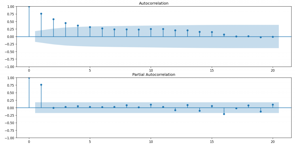
## 從acf 和pacf 圖『主觀地』決定我們arima 的d和p要設置多少
fig = plt.figure(figsize=(12,8))
ax1 = fig.add_subplot(211)
fig = sm.graphics.tsa.plot_acf(df_order, lags=20,ax=ax1)
ax1.xaxis.set_ticks_position('bottom')
fig.tight_layout()
ax2 = fig.add_subplot(212)
fig = sm.graphics.tsa.plot_pacf(df_order, lags=20, ax=ax2)
ax2.xaxis.set_ticks_position('bottom')
fig.tight_layout()
plt.show()

Step 5. Build the ARIMA Model

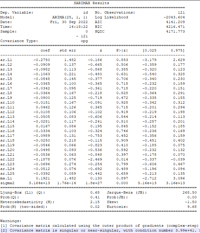
# 搭建ARIMA Model
model = sm.tsa.arima.ARIMA(df_order, order=(25,1,1))## p 設定和前n筆資料趨勢有關，d設定為1，q設定為1
model_fit = model.fit()
print(model_fit.summary())

Step 6. Plot residual errors

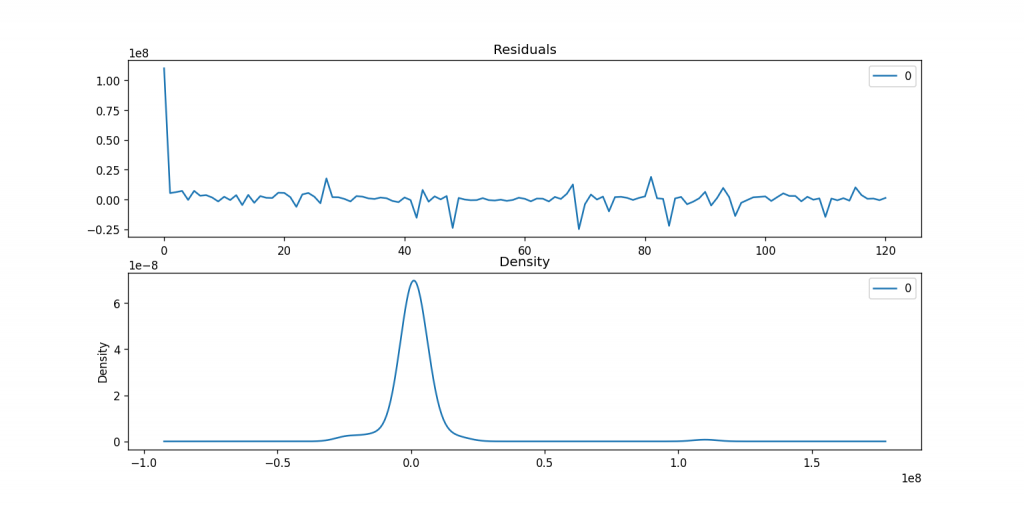
## 重點關注指標，1.P值，2. coef
# Plot residual errors
residuals = pd.DataFrame(model_fit.resid)
fig, ax = plt.subplots(2,1)
residuals.plot(title="Residuals", ax=ax[0])
residuals.plot(kind='kde', title='Density', ax=ax[1])
plt.show()

Step 7. Print the prediction (result)

### 輸出模型預測結果
prediction = model_fit.predict(1,150,dynamic=False)
print(prediction)

Step 8. Concate the results

## 組裝訓練＋期望預測數據
df_filter_test_2_2_1 = df_order.append(df_test,ignore_index=True)
print(df_filter_test_2_2_1)

Step 9. Visualation of the results

## 視覺化
#visualize 
fig, ax = plt.subplots(figsize=(8, 5))
ax.plot(prediction,label = 'prediction',linestyle='--',color = 'red')
ax.plot(df_filter_test_2_2_1[120:150],label = 'real_order_202204', color = 'green')
ax.plot(df_order,label = 'real_history_data', color = 'gray',linestyle=':')
ax.set_xlabel('timestamp')  # Add an x-label to the axes.
ax.set_ylabel('order count')  # Add a y-label to the axes.
ax.set_title("order_predict")  # Add a title to the axes.
ax.legend();  # Add a legend.

Result & Graph

Other reference of ARIMA: (full code)

#!/usr/bin/python

import numpy as np
import pandas as pd
import matplotlib.pyplot as plt
from statsmodels.tsa.arima_model import ARIMA


def date_parse(date):
    return pd.datetime.strptime(date, '%Y-%m')

if __name__ == '__main__':

    data = pd.read_csv('AirPassengers.csv', header = 0, parse_dates = ['Month'], date_parser = date_parse, index_col = ['Month'])
    p,d,q = 2, 1, 2
    data.rename(columns = {'#Passengers':'Passengers'}, inplace = True)
    passengersNums = data['Passengers'].astype(np.float)
    logNums = np.log(passengersNums)
    subtractionNums = logNums - logNums.shift(periods = d)
    rollMeanNums = logNums.rolling(window = q).mean()
    logMRoll = logNums - rollMeanNums

    plt.plot(logNums, 'g-', lw = 2, label = u'log of original')
    plt.plot(subtractionNums, 'y-', lw = 2, label = u'subtractionNums')
    plt.plot(logMRoll, 'r-', lw = 2, label = u'log of original - log of rollingMean')
    plt.legend(loc = 'best')
    plt.show()

    arima = ARIMA(endog = logNums, order = (p,d,q))
    proArima = arima.fit(disp = -1)
    fittedArima = proArima.fittedvalues.cumsum() + logNums[0]
    fittedNums = np.exp(fittedArima)
    plt.plot(passengersNums, 'g-', lw = 2, label = u'orignal')
    plt.plot(fittedNums, 'r-', lw = 2, label = u'fitted')
    plt.legend(loc = 'best')
    plt.show()

Furthermore:

The other reference codes of ARIMA (full code) can refer to THIS LINK