單源對短路徑問題(single source shortest path problem, sssp)為給一個vertex(called source)，找到去圖上其他節點的最短距離，其有三種解法 1. Breadth First Search (BFS) 2. Dijkstra’s Algorithm 3. Bellman Ford。(Depth First Search(DFS)無法解SSSP，因其一開始就走遠了......)。但BFS無法用來解有權重的圖(weighted graph)，這時，我們會使用Dijskstra’s algorithm。

Solve unweighted graph SSSP problem with BFS

首先我們先來看用BFS解SSSP問題，下面範例可以搭配圖一起看: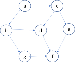

圖1，譬如說在下面的例子中我們想看a->e的最短路徑，那麼做法就是先走一步，可以是a->c，或是a->b，b和c都不是終點，所以再走一步，可以是a->b->g, a->b->d,a->c->d, a->c->e，而e為終點，回傳a->c->e程式碼結束。Done!

from collections import deque, defaultdict

class Graph:
    def __init__(self, input=None):
        if input == None:
            self.gdict = defaultdict(list)
        else:
            self.gdict = input

    def __str__(self):
        res = ''
        for key, value in self.gdict.items():
            res += f'{key}:{value}\n'
        return res
        
    # time complexity: O(E), space complexity: O(E)
    # 這裡其實就是用breadth first search 的方式，一層一層的走出來，先到終點的那條路即是最短路徑
    def BFS_SSSP(self, start, end):
        queuepath = deque()
        queuepath.append([start])
        while len(queuepath) != 0:
            path = queuepath.popleft()
            node = path[-1]
            if node == end:
                return path
            for i in self.gdict.get(node, []):
                new_path = list(path)
                new_path.append(i)
                queuepath.append(new_path)


customDict = {'a': ['b', 'c'], 'b': ['d', 'g'], 'c': ['d', 'e'], 'd': ['f'], 'e': ['f'], 'g': ['f']}
mygraph = Graph(customDict)
print(mygraph.BFS_SSSP('a', 'e'))
>> ['a', 'c', 'e']
## 這裡我們得出a到e的最短路徑為a -> c -> e

Solve weighted graph SSSP with Dijkstra’s algorithm

猶如我們前面提到BFS無法用在weighted graph上，接著我們來介紹Dijkstra's algorithm。Dijkstra's algorithm也是用來解決單源路徑問題，它weighted graph和unweighted graph都可以解決，它的計算算是一種貪婪算法(greedy algorithm)，從下面的程式碼/圖我們可以發現，我們不斷為每個點找局部最小值(局部最佳解)，並標註為visited，一直到所有節點都被標註完。一般來說貪婪算法找到的局部最佳解未必是全域最佳解，但在使用Dijkstra's algorithm上的限制:邊(edge)的權重(weight)不能為負，使找出來的局部最佳解可以為全域最佳解，我們直接用圖和表格來說明可能更好理解: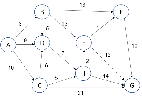

圖2 今天我們有個directed weight graph，我們想從A出發，然後找到到各點的最短距離
那我們可以follow 以下表格，首先創建一個表格，有選項visited、node(節點)、到初始點最小距離、predecessor(前一個節點)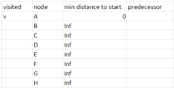

Step 0 由A開始，設其餘到A點距離無限大(Inf)，A自己到自己0，A為最小值，標記為visited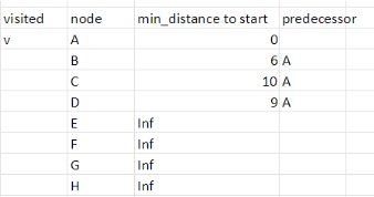

step 1 A可以到B,D,C:0+edge分別為6,9,10，皆小於Inf，更新表格並填A為他們的前一個節點。此時B為為標記的點裡最小，標記B為visited。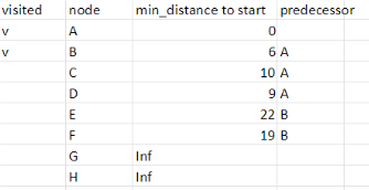

Step 2 B點可以到D, E, F。D: 6+5=11>9 不用更新，E:6+16=22小於Inf 更新，F:6+13=19小於Inf更新。同樣的方式以此類推......
Step 3 細節參考表格右邊小小的計算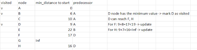

Step 4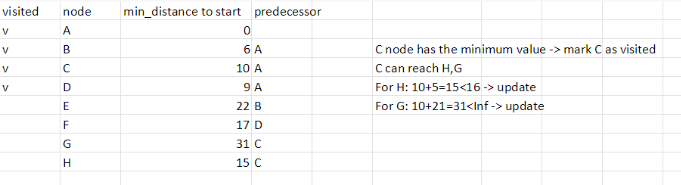

Step 5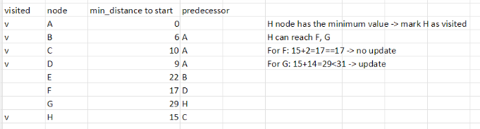

Step 6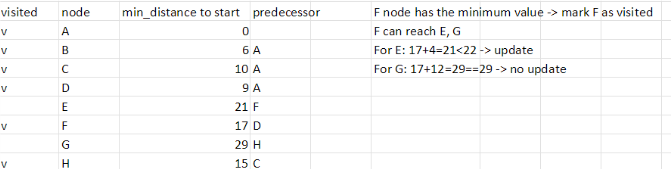

Step 7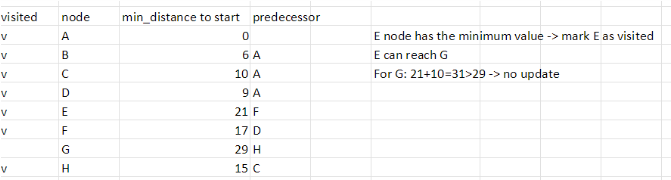

所以如果我們想知道起始點A到某一點的最短路徑，我們可以從predecessor推回去，舉例來說，如果我們想找A到H最短路徑: H<-C<-A， 根據表格最短路徑就會是15，以此類推。接著我們來看程式碼:

import heapq

class Edge:
    def __init__(self, v1, v2, w):
        self.weight = w
        self.start_vertex = v1
        self.target_vertex = v2
# 這裡我們預設所有min_distance無限大，之後再來更新
# 然後用neightbors來append edge
class Node:
    def __init__(self, v1):
        self.name = v1
        self.neighbors = []
        self.min_distance = float('Inf')
        self.visited = False
        self.predecessor = None
# 這個是python class內建<符號對應的function，那這裡我們是要讓不同節點間的min_distance去做比較
    def __lt__(self, other):
        return self.min_distance < other.min_distance

    def add_edge(self, w, v2):
        new_edge = Edge(self, v2, w)
        self.neighbors.append(new_edge)

# 這裡計算的概念跟我們文章前面講的一樣，這裡就不再贅述，大家可以自己看一遍後實作一遍
class Dijkstra:
    def __init__(self, start=None):
        self.heap = []
        self.start = start

    def calculate(self, start):
        self.start = start
        start.min_distance = 0
        heapq.heappush(self.heap, start)
        while self.heap:
            current_vertex = heapq.heappop(self.heap)
            if current_vertex.visited:
                continue
            for edge in current_vertex.neighbors:
                start_vertex = edge.start_vertex
                target_vertex = edge.target_vertex
                new_distance = current_vertex.min_distance+edge.weight
                if new_distance < target_vertex.min_distance:
                    target_vertex.min_distance = new_distance
                    target_vertex.predecessor = start_vertex
                    heapq.heappush(self.heap, target_vertex)
            current_vertex.visited = True

    def find_shortest_path(self, end):
        print(
            f'The shortest path from {self.start.name} to {end.name} is {end.min_distance}')
        route = []
        current = end
        while current:
            route.append(current.name)
            current = current.predecessor
        route.reverse()
        print('->'.join(route))


nodeA = Node('A')
nodeB = Node('B')
nodeC = Node('C')
nodeD = Node('D')
nodeE = Node('E')
nodeF = Node('F')
nodeG = Node('G')
nodeH = Node('H')
nodeA.add_edge(6, nodeB)
nodeA.add_edge(10, nodeC)
nodeA.add_edge(9, nodeD)
nodeB.add_edge(16, nodeE)
nodeB.add_edge(5, nodeD)
nodeB.add_edge(13, nodeF)
nodeC.add_edge(6, nodeD)
nodeC.add_edge(5, nodeH)
nodeC.add_edge(21, nodeG)
nodeD.add_edge(8, nodeF)
nodeD.add_edge(7, nodeH)
nodeE.add_edge(10, nodeG)
nodeF.add_edge(12, nodeG)
nodeF.add_edge(4, nodeE)
nodeH.add_edge(2, nodeF)

example = Dijkstra()
example.calculate(nodeA)
example.find_shortest_path(nodeE)
>> The shortest path from A to E is 21
   A->D->F->E

Bellman-Ford algorithm for SSSP

我們前面提到，當權重(weight)為負的時，我們無法使用Dijkstra's algorithm，於是接下來我們要介紹Bellman- Ford algorithm，我感覺把這個放在這篇講感覺會比較連貫。Bellman-Ford Algorithm也是用來解決單源最短路徑問題，其也是可以用在weighted和unweighted graphs. 它可以解決Dijkstra’s algorithm 解決不了的negative edge weights graph(圖裡有邊的權重為負的)。但其仍無法解決有負循環途徑(negative cycle)的圖(也就是圖裡有一個cycle(循環途徑)，其權重總和為負值)，因為如果我們重複無限次的去走這個負循環途徑，算出來的值可以持續無限制的降低。雖然Bellman-Ford無法計算有負循環途徑的圖，但Bellman-Ford能夠判斷圖裡是否有負循環途徑。

那判斷的方法如下，假設我們在圖中有N個節點，那麼要算得單源最短路徑，總共最多N-1次的更新最短路徑。(N-1的原因是，如果我們有N個節點，我們最多就只N-1個邊(edges)，讓每個邊都走過一遍)。如果我們走第N次，最短路徑(shortest distance)還在被更新，那麼我們說這個graph裡面有negative cycle。以下我們看程式碼比較快，我覺得Bellman-Ford比Dijkstra 來得好理解:

class Graph:
   # 初始化graph，NumV:vertice的數目
    def __init__(self):
        self.NumV = 0
        self.graph = []
        self.node = []
   # 增加節點
    def add_node(self, vertice):
        self.node.append(vertice)
        self.NumV += 1
   # 增加邊
    def add_edge(self, start, target, weight):
        self.graph.append([start, target, weight])
    # bellmanford algorithm: 我們選起始點
    def bellmanford(self, source):
        # 創建distance字典
        # 一開始我們設所有結點的min distance為Inf
        mydict = {i: float('Inf') for i in self.node}
        # 起始點min distance為0
        mydict[source] = 0
        # 我們需要更新比較n-1次
        for _ in range(self.NumV-1):
            for start, target, weight in self.graph:
                if mydict[start] != 'Inf' and mydict[start]+weight < mydict[target]:
                    mydict[target] = mydict[start]+weight
        # 如果過了n-1次 它還在更新，那麼圖裡肯定有negative cycle
        if mydict[start] != 'Inf' and mydict[start]+weight < mydict[target]:
            return 'The graph contains a negative cycle'
        else:
            res = ''
            for key, value in mydict.items():
                res += f'{key}:{value}\n'
            return res


g = Graph()
g.add_node('A')
g.add_node('B')
g.add_node('C')
g.add_node('D')
g.add_node('E')
g.add_edge('A', 'C', 6)
g.add_edge('A', 'D', 6)
g.add_edge('B', 'A', 3)
g.add_edge('C', 'D', -1)
g.add_edge('D', 'C', 2)
g.add_edge('D', 'B', 1)
g.add_edge('E', 'B', 4)
g.add_edge('D', 'E', 2)
print(g.bellmanford('A'))
>>  A:0
    B:6
    C:6
    D:5
    E:7
# 得到從A點出發到各點的最短距離!

參考資料:
The Complete Data Structures and Algorithms Course in Python (Udemy)
https://www.geeksforgeeks.org/bellman-ford-algorithm-dp-23/