邏輯迴歸 (Logistic Regression)

分類度量

混淆矩陣（Confusion Matrix）

混淆矩陣包括真正例（True Positives, TP）、假正例（False Positives, FP）、真負例（True Negatives, TN）、和假負例（False Negatives, FN）。

準確率（Accuracy）

正確預測的樣本數除以總樣本數的比例

• Accuracy = TP+TN/TP+FP+TN+FN

錯誤率（Error Rate）

錯誤預測的樣本數除以總樣本數的比例

• Error Rate = FP+FN/TP+FP+TN+FN

精確率（Precision）

被模型預測為正類別的樣本中，實際為正類別的比例

• Precision = TP/TP+FP

召回率（Recall）

實際為正類別的樣本中，被模型預測為正類別的比例

• Recall = TP/TP+FN

F1-Score

精確率和召回率的調和平均，用於綜合評估分類模型的性能

• F1-Score = 2⋅Precision⋅Recall/Precision+Recall

ROC曲線（Receiver Operating Characteristic Curve）

• 評估二元分類模型性能
• 假陽率（False Positive Rate, FPR）為橫軸
• 真陽率（True Positive Rate, TPR）為縱軸
• AUC（Area Under Curve）為ROC曲線下方的面積，通常用於度量模型的性能。AUC的值在0.5到1之間，越接近1表示模型性能越好。

KS曲線（Kolmogorov-Smirnov曲線）

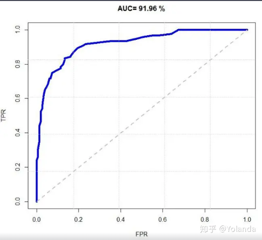
評估二元分類模型的風險區分能力。KS值越大，模型的風險區分能力越強。

Lift值

評估模型的預測效果，它比較了使用模型和隨機選擇的效果。Lift值大於1表示模型的預測效果較好。

PR曲線（Precision-Recall Curve）

精確率和召回率之間的關係，尤其在不平衡類別問題中很有用。

邏輯回歸實作

• Python

import pandas as pd
from sklearn.model_selection import train_test_split
from sklearn.linear_model import LogisticRegression
from sklearn.metrics import accuracy_score, confusion_matrix
import seaborn as sns
import matplotlib.pyplot as plt

# 載入資料集
iris = sns.load_dataset('iris')

# 前處理資料
# 分離出了特徵變數 X 和目標變數 y。
# species 列（即花的種類）作為目標變數並將其從特徵變數中刪除
X = iris.drop('species', axis=1)
y = iris['species']

# 切分資料集為訓練集和測試集 (70% 訓練，30% 測試)
# 資料集被分成了 X_train、X_test、y_train 和 y_test 四個部分。
# 訓練70%、測試30%
# random_state=任意數字(seed)
X_train, X_test, y_train, y_test = train_test_split(X, y, test_size=0.3, random_state=123)

# 建立邏輯回歸模型
model = LogisticRegression()
model.fit(X_train, y_train)

# 在測試集上進行預測
predictions = model.predict(X_test)

# 評估模型性能
accuracy = accuracy_score(y_test, predictions)
print("準確率：", accuracy)

# 繪製混淆矩陣
confusion = confusion_matrix(y_test, predictions)
print("混淆矩陣：")
print(confusion)

# 預測結果與實際結果的比較圖
comparison_df = pd.DataFrame({'Actual': y_test, 'Predicted': predictions})
comparison_plot = sns.countplot(data=comparison_df, x='Actual', hue='Predicted')
comparison_plot.set_title('Predicted and Actual')
plt.show()

準確率： 0.9333333333333333
混淆矩陣：
[[18 0 0]
[ 0 10 0]
[ 0 3 14]]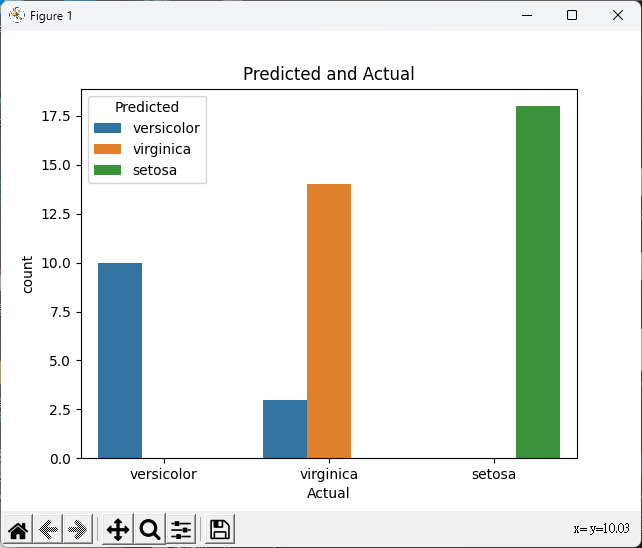

• R

# 載入必要的套件
library(ggplot2)
library(dplyr)
library(ggpubr)

# 使用內建的 iris 資料集
data(iris)

# 前處理資料
iris <- iris %>%
  mutate(Species = as.factor(Species))  # 將目標變數轉為因子型態

# 切分資料集為訓練集和測試集 (70% 訓練，30% 測試)
set.seed(123)
train_indices <- sample(1:nrow(iris), 0.7 * nrow(iris))
train_data <- iris[train_indices, ]
test_data <- iris[-train_indices, ]

# 建立邏輯回歸模型
model <- glm(Species ~ Sepal.Length + Sepal.Width + Petal.Length + Petal.Width, 
             data = train_data, family = binomial)

# 在測試集上進行預測
predictions <- predict(model, newdata = test_data, type = "response")
predicted_classes <- ifelse(predictions > 0.5, "versicolor", "setosa")

# 評估模型性能
accuracy <- sum(predicted_classes == test_data$Species) / nrow(test_data)
cat("準確率：", accuracy, "\n")

# 繪製混淆矩陣
confusion_matrix <- table(predicted_classes, test_data$Species)
cat("混淆矩陣：\n")
print(confusion_matrix)

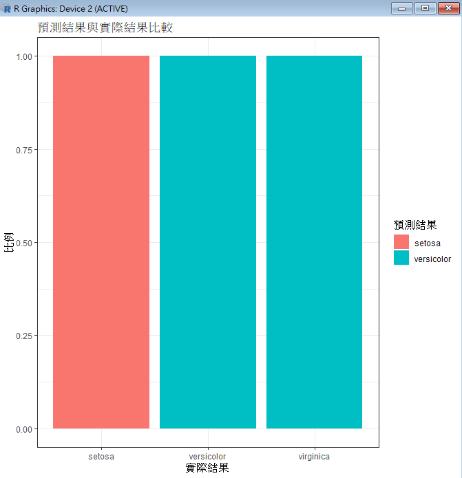
# 繪製預測結果與實際結果的比較圖
comparison_plot <- ggplot(test_data, aes(x = Species, fill = predicted_classes)) +
  geom_bar(position = "fill") +
  labs(title = "預測結果與實際結果比較", x = "實際結果", y = "比例", fill = "預測結果") +
  theme_bw()
print(comparison_plot)

多分類問題

宏平均（Macro-Average）

計算每個類別的性能指標（如精確率和召回率）的平均值。首先計算每個類別的指標，然後取平均值。

微平均（Micro-Average）

微平均計算全局混淆矩陣的性能指標，不考慮類別。首先計算全局混淆矩陣的指標，然後計算性能指標。

Kappa係數（Cohen's Kappa）

Kappa係數用於衡量模型在多分類問題中的性能，考慮了隨機預測的效果。值越高表示模型性能越好，通常在0到1之間。