決策樹

• 用於分類和回歸問題。

混亂評估指標

• Information Gain (資訊獲利)
  • 衡量了使用某個特徵分割後熵的減少
  • 熵是衡量不確定性的指標。
• Gain ratio (吉尼獲利)
  • Information Gain的一種變體
  • 考慮到特徵的分支數量，以避免過多的分支
• Gini index (吉尼係數) = Gini Impurity (吉尼不純度)
  • 測量了在某個節點上隨機選擇一個類別標籤並錯誤分類的機率。
  • Gini Impurity越低，節點的純度越高。

超參數調整

• 最大深度
• 最小樣本分割
• 節點最小樣本數等等

評估分割資訊量

• 資訊獲利 (Information Gain)
• Gini不純度 (Gini Impurity)
• 評估分割資訊量

熵 (Entropy)

• 計算Information Gain的一種方法。
• 分類一致時，熵為0，當資料各有一半不同時，熵為1。
• 0~1，越少越好(接近0)

資訊增益(Information Gain)

• 決策樹分割特徵的度量
• 在某個節點上使用特定特徵進行分割後，熵的減少程度
• 資訊增益越高，特徵的選擇對於分類的影響越大

Gini 不純度 (Gini Impurity)

• 另一種評估分割資訊量的方法。
• 分類一致時，Gini不純度為0，當資料各有一半不同時，Gini不純度為0.5。

決策樹模型的優缺點

Pros

• 易於理解和解釋
• 能處理數值和分類特徵
• 不需要太多的數據預處理

Cons

• 容易過擬合
• 對噪聲敏感
• 在處理某些複雜問題上表現不佳，因為它們只能生成分段線性模型。對於非線性問題，要用更複雜的模型

迴歸樹

• 樹的深度影響模型的複雜度，深度越深，模型越複雜。
• 切割點
  迴歸樹使用均方差（MSE）或平均絕對誤差（MAE）來評估模型，找出誤差最小的值作為切割點。
  • CART 決策樹 (Classification and Regression Tree)
  • CART決策樹可用於分類和回歸問題，採用二分法。

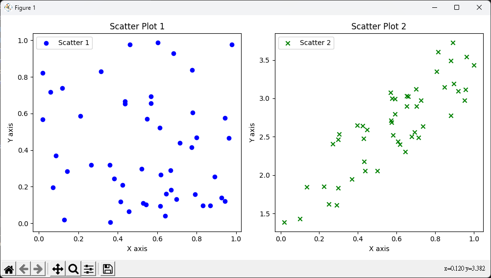
散點圖

import matplotlib.pyplot as plt
import numpy as np

# 第一組隨機數據
np.random.seed(0)
x1 = np.random.rand(50)
y1 = np.random.rand(50)

# 第二組隨機數據（線性相關）
x2 = np.random.rand(50)
y2 = 2 * x2 + 1 + np.random.rand(50)


plt.figure(figsize=(10, 5)) 

plt.subplot(1, 2, 1) 
plt.scatter(x1, y1, label='Scatter 1', color='blue', marker='o')
plt.xlabel('X axis')
plt.ylabel('Y axis')
plt.title('Scatter Plot 1')
plt.legend()

plt.subplot(1, 2, 2)  
plt.scatter(x2, y2, label='Scatter 2', color='green', marker='x')
plt.xlabel('X axis')
plt.ylabel('Y axis')
plt.title('Scatter Plot 2')
plt.legend()

plt.tight_layout() 
plt.show()

實作

import numpy as np
import matplotlib.pyplot as plt
from sklearn.tree import DecisionTreeRegressor
from sklearn import linear_model

# 資料集
x = np.array(list(range(1, 11))).reshape(-1, 1)
y = np.array([4.50, 4.75, 4.91, 5.34, 5.80, 7.05,
             7.90, 8.23, 8.70, 9.00]).ravel()

# 建立迴歸模型
model1 = DecisionTreeRegressor(max_depth=1)
model2 = DecisionTreeRegressor(max_depth=3)
model3 = linear_model.LinearRegression()
model1.fit(x, y)
model2.fit(x, y)
model3.fit(x, y)

# 預測
X_test = np.arange(0.0, 10.0, 0.01)[:, np.newaxis]
y_1 = model1.predict(X_test)
y_2 = model2.predict(X_test)
y_3 = model3.predict(X_test)

plt.figure()
plt.scatter(x, y, s=20, edgecolor="black",
            c="darkorange", label="data")
plt.plot(X_test, y_1, color="cornflowerblue",
         label="max_depth=1", linewidth=2)
plt.plot(X_test, y_2, color="yellowgreen", label="max_depth=3", linewidth=2)
plt.plot(X_test, y_3, color='red', label='liner regression', linewidth=2)
plt.xlabel("data")
plt.ylabel("target")
plt.title("Decision Tree Regression")
plt.legend()

plt.text(0.5, 8.5, "max_depth=1: Underfitting", fontsize=10, color="blue")
plt.text(4.5, 4.5, "max_depth=3: Balanced", fontsize=10, color="green")
plt.text(6.0, 9.0, "Linear Regression", fontsize=10, color="red")

plt.show()

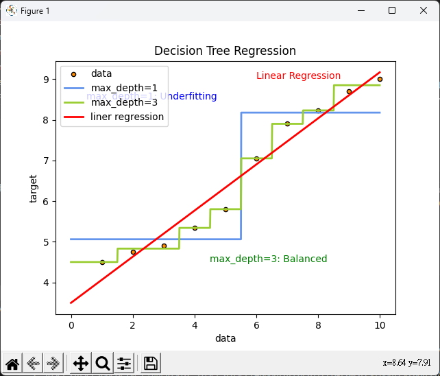
• 藍色曲線（max_depth=1）：
  • 這是深度為1。
  • 只有一個節點，一個預測值。
• 綠色曲線（max_depth=3）：
  • 深度3表示樹有3個節點。
  • 模型比較複雜，可以更好地擬合資料。
• 紅色曲線（linear regression）：
  • 線性回歸模型的預測結果。
  • 建立一條直線來擬合資料。
• x軸：
  • x軸表示輸入特徵（data）
  • 範圍從0到10，這是用來進行預測的輸入範圍。
• y軸：
  • y軸表示目標變數（target）
  • 預測的輸出值。

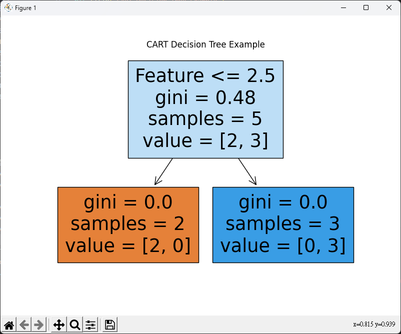
CART 決策樹 (Classification and Regression Tree)

• 二分法
• 在每個節點上，將數據分為兩個子節點
• 一個包含特定特徵值，另一個則不包含

from sklearn.tree import plot_tree
import numpy as np
from sklearn.tree import DecisionTreeClassifier, DecisionTreeRegressor
import matplotlib.pyplot as plt

X = np.array([[1.0], [2.0], [3.0], [4.0], [5.0]])
y = np.array([0, 0, 1, 1, 1])  # 目標類別

# CART分類樹模型
clf = DecisionTreeClassifier()
clf.fit(X, y)

# 預測新數據點的類別
new_data_point = np.array([[3.5]])
predicted_class = clf.predict(new_data_point)
print(f"Predicted class for {new_data_point}: {predicted_class}")

# 繪製決策樹
plt.figure(figsize=(8, 6))
plot_tree(clf, filled=True, feature_names=['Feature'])
plt.title("CART Decision Tree Example")
plt.show()

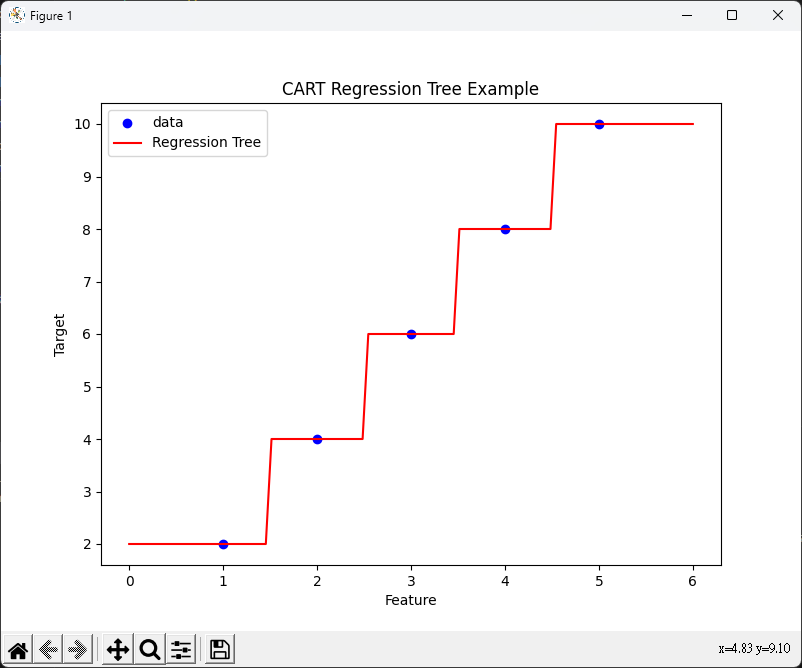
# 生成另一個示例數據集（這是回歸的示例）
X_reg = np.array([[1.0], [2.0], [3.0], [4.0], [5.0]])
y_reg = np.array([2.0, 4.0, 6.0, 8.0, 10.0])  # 這是目標回歸值

# CART回歸樹模型
reg = DecisionTreeRegressor()

# 適合（fit）模型使用數據
reg.fit(X_reg, y_reg)

# 預測新數據點的回歸值
new_data_point_reg = np.array([[3.5]])
predicted_value = reg.predict(new_data_point_reg)
print(f"Predicted value for {new_data_point_reg}: {predicted_value}")

# 繪製回歸樹
plt.figure(figsize=(8, 6))
plt.scatter(X_reg, y_reg, c="b", label="data")
plt.plot(np.linspace(0, 6, 100)[:, np.newaxis], reg.predict(
    np.linspace(0, 6, 100)[:, np.newaxis]), color="r", label="Regression Tree")
plt.xlabel("Feature")
plt.ylabel("Target")
plt.legend()
plt.title("CART Regression Tree Example")
plt.show()