7. 如何有效率找出最佳的w和b
   可以利用gradient descent(梯度下降)，也就是根據斜率去改變參數
   原本的cost = (真實數據-預測值)^2，也就是cost = (y-y_pred)^2，若將y_pred = w．x + b，且b假設為0帶入，可以得到(y-wx)^2，若將其微分，則可以知道切線斜率，就能利用gradient descent(梯度下降)來找出最佳的組合(切線斜率相當接近0)。

• 導入檔案

import pandas as pd
url = "https://raw.githubusercontent.com/GrandmaCan/ML/main/Resgression/Salary_Data.csv"
data = pd.read_csv(url)

x = data["YearsExperience"]
y = data["Salary"]

• 計算cost

def compute_cost(x, y, w, b):
    y_pred = w*x + b
    cost = (y - y_pred)**2
    cost =  cost.sum() / len(x) 

    return cost

• 計算gradient

def compute_gradient(x, y, w, b):
    w_gradient = (2*x*(w*x+b - y)).mean() #對w微分後計算平均值
    b_gradient = (2*(w*x+b - y)).mean() #對b微分後計算平均值
    return w_gradient, b_gradient

• 學習率(learning rate)：控制模型中梯度下降的速度

w = 0
b = 0
learning_rate = 0.001
w_gradient, b_gradient = compute_gradient(x, y, w, b)
print(compute_gradient(x, y, w, b))

w = w - w_gradient*learning_rate
b = b - b_gradient*learning_rate
print(compute_gradient(x, y, w, b))
＃輸出：
6040.596363636363
5286.0782714844245

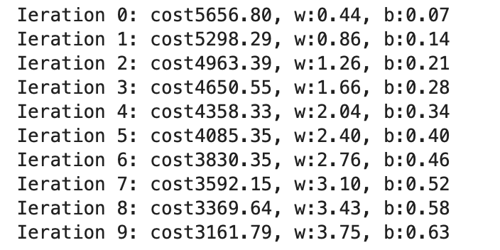
=>執行10次

w = 0
b = 0
learning_rate = 0.001
for i in range(10):
    w_gradient, b_gradient = compute_gradient(x, y, w, b)
    w = w - w_gradient*learning_rate
    b = b - b_gradient*learning_rate 
    
    cost =  compute_cost(x, y, w, b)
    print(f"Ieration {i}: cost{cost}, w:{w:.2f}, b:{b:.2f}")

=>執行10000次，每1000次print一次結果

w = 0
b = 0
learning_rate = 0.001
for i in range(10000):
    w_gradient, b_gradient = compute_gradient(x, y, w, b)
    w = w - w_gradient*learning_rate
    b = b - b_gradient*learning_rate 
    
    cost =  compute_cost(x, y, w, b)
    if i%1000 == 0:
        print(f"Ieration {i:5}: cost{cost: .2e}, w:{w: .2e}, b:{b: .2e}, w_gradient:{w_gradient: .2e}, b_gradient:{b_gradient: .2e}")

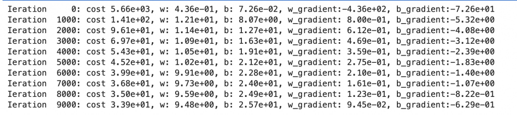
(可以看到cost依舊有在下降，但幅度有越來越小的趨勢，斜率gradient越來越接近0)

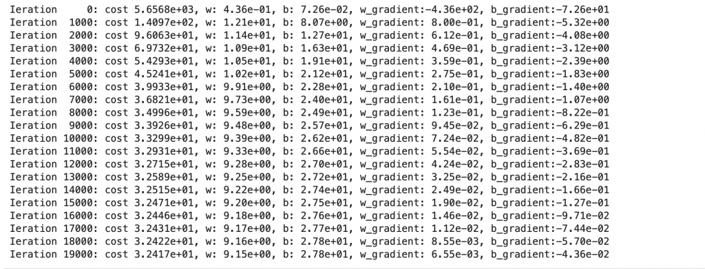
=>寫成函式：

def gradient_descent(x, y, w_init, b_init,  learning_rate,  cost_function, gradient_function,  run_iter, p_iter=1000): 
    c_hist = []
    w_hist = []
    b_hist = [] 
    
    w = w_init
    b = b_init
     
    for i in range(run_iter ):
        w_gradient, b_gradient = gradient_function (x, y, w, b)
        
        w = w - w_gradient*learning_rate
        b = b - b_gradient*learning_rate 
        cost =  cost_function(x, y, w, b)

        w_hist.append(w)
        b_hist.append(b)
        c_hist.append(cost)
         
        if i%p_iter == 0:
            print(f"Ieration {i:5}: cost{cost: .4e}, w:{w: .2e}, b:{b: .2e}, w_gradient:{w_gradient: .2e}, b_gradient:{b_gradient: .2e}")

    return w, b, w_hist, b_hist, c_hist

執行看看：

w_init = 0
b_init = 0
learning_rate = 1.0e-3
run_iter = 20000

w_final, b_final, w_hist, b_hist, c_hist = gradient_descent(x, y, w_init, b_init,  learning_rate,  compute_cost, compute_gradient,  run_iter)

圖示：

import matplotlib.pyplot as plt
import numpy as np

plt.plot(np.arange(0, 20000), c_hist)
plt.title("itertion vs cost")
plt.xlabel("itertion")
plt.ylabel("cost")
plt.show()

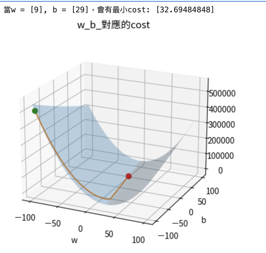
=>設定不同初始點，gradient descend的路徑：

w_init = -100
b_init = -100
learning_rate = 1.0e-3
run_iter = 20000

w_final, b_final, w_hist, b_hist, c_hist = gradient_descent(x, y, w_init, b_init,  learning_rate,  compute_cost, compute_gradient,  run_iter)

w_index, b_index = np.where(costs == np.min(costs))
print(f"當w = {ws[w_index]}, b = {bs[b_index]}，會有最小cost: {costs[w_index, b_index]}")

ax = plt.axes(projection = "3d")
ax.view_init(20, - 65)
plt.figure(figsize =  (7,7))

b_grid, w_grid = np.meshgrid(bs, ws)

ax.plot_surface(w_grid, b_grid, costs, alpha = 0.3)
ax.scatter(ws[w_index], bs[b_index], costs[w_index, b_index], color = "red", s = 40)
ax.scatter(w_hist[0], b_hist[0], c_hist[0], color = "green", s = 40)
ax.plot(w_hist, b_hist, c_hist)
ax.set_title("w_b_對應的cost")
ax.set_xlabel("w")
ax.set_ylabel("b")
plt.show()

學習資料來源：GrandmaCan -我阿嬤都會

機器學習的過程：準備資料=>設定模型=>設定cost function=>設定optimizer