前言
昨天我們完成了邏輯迴歸模型的建立與深入分析，包括特徵權重與混淆矩陣評估。
今天學習重點包括：

• 理解邏輯迴歸主要超參數
• 使用交叉驗證評估模型穩定性
• 比較不同參數設定對模型表現的影響
  透過今天的分析，我們可以更穩定地預測未見資料，並了解不同參數設定對模型的影響。

一、邏輯迴歸主要超參數介紹

• C（正則化強度倒數）
  • 說明：控制正則化強度，C 值越小正則化越強
  • 作用：防止模型過度擬合，權重不會過大
  • 設定示例：C=1.0 為預設值，C=0.1 強正則化，C=10 弱正則化
• penalty（正則化類型）
  • 說明：L1 或 L2 正則化
  • L1 可做特徵篩選（部分權重會變 0）
  • L2 保持所有特徵但限制權重大小
• max_iter（最大迭代次數）
  • 說明：模型優化時最多迭代次數
  • 作用：確保梯度下降收斂
  • 示例：max_iter=500 可避免收斂警告
• solver（優化算法）
  • 說明：選擇算法求解邏輯迴歸
  • 示例：lbfgs 適合中小資料、liblinear 適合小資料與 L1 正則化

為什麼要調參數？

• 超參數會影響模型的學習能力與泛化能力
• 適當的正則化可以降低過擬合風險
• 不同 solver 對大資料或稀疏資料效率不同

二、使用交叉驗證評估模型
交叉驗證（Cross-Validation）

• 將資料分成 k 份，每次用 1 份做驗證，其他做訓練，重複 k 次
• 最後取平均結果，得到穩定評估
• 公式：
  
  程式碼示範

from sklearn.model_selection import cross_val_score
from sklearn.linear_model import LogisticRegression

# 建立模型
model = LogisticRegression(max_iter=500, C=1.0, penalty='l2', solver='lbfgs')

# 5-fold 交叉驗證
scores = cross_val_score(model, X_train, y_train, cv=5, scoring='accuracy')

print("每折準確率:", scores)
print("平均準確率:", scores.mean())

程式碼解釋

• cross_val_score 自動分折、訓練與驗證
• scores 保存每折準確率，scores.mean() 計算平均準確率
• 這樣比單次測試集更穩定可靠

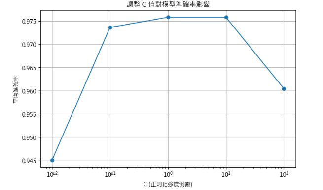
三、視覺化不同 C 值對準確率影響

import matplotlib.pyplot as plt

C_values = [0.01, 0.1, 1, 10, 100]  # 嘗試不同正則化強度
mean_scores = []

for C in C_values:
    # 建立模型，僅改變 C
    model = LogisticRegression(max_iter=500, C=C, penalty='l2', solver='lbfgs')
    scores = cross_val_score(model, X_train, y_train, cv=5)
    mean_scores.append(scores.mean())

plt.figure(figsize=(8,5))
plt.plot(C_values, mean_scores, marker='o')
plt.xscale('log')  # 對數刻度，更直觀
plt.xlabel('C (正則化強度倒數)')
plt.ylabel('平均準確率')
plt.title('調整 C 值對模型準確率影響')
plt.grid(True)
plt.show()

解釋

• C 值越小 → 強正則化 → 權重較小，模型較簡單
• C 值越大 → 弱正則化 → 權重自由，模型較複雜
• 折線圖顯示平均準確率，幫助找到最佳 C
  

小結
今天我們學習了邏輯迴歸的主要超參數，包括 C 值、正則化類型、最大迭代次數以及求解器（solver），並透過交叉驗證了解模型在未見資料上的穩定性。此外，我們還視覺化了不同 C 值對平均準確率的影響，幫助找到最佳的正則化設定。透過這些操作，我們不僅能調整模型參數，也對模型的學習能力與泛化能力有初步認識。後續章節中，我們將進一步解釋這些專有名詞，包括正則化、梯度以及優化算法，並搭配簡單數學例子，讓今天學到的超參數調整背後原理更加清楚。